PEIBOS-CAPD

When compiling CODAC with the codac-capd extension (see here), the CAPD version of the PEIBOS library is also compiled.

Let us consider an initial set \(\mathbb{X}_0 \subset \mathbb{R}^n\) with its boundary \(\partial \mathbb{X}_0\). Considering a dynamical system \(\dot{\mathbf{x}}=\gamma(\mathbf{x})\), the PEIBOS tool allows to compute the reach set \(\mathbf{X}_t=\left\{ \mathbf{x}(t) \mid \mathbf{x} \in \partial \mathbb{X}_0 \right\}\).

Gnomonic atlas

To handle the boundary of the initial set \(\mathbb{X}_0\), the PEIBOS tool relies on a gnomonic atlas. See Gnomonic atlas.

Use

The computation of the reach set is decomposed into two separate functions.

PEIBOS

The PEIBOS function takes at least six arguments :

The CAPD IMap representing \(\gamma\).
The final time for the integration of the ODE.
A timestep to get intermediate states.
The inverse chart for the gnomonic atlas (an analytic function).
The list of symmetries for the gnomonic atlas. Note that each symmetry is represented as a hyperoctahedral symmetry, see sec-actions-octasym.
A resolution \(\epsilon\). The initial box \(\left[-1,1\right]^m\) will initiallly be splitted in boxes with a diameter smaller than \(\epsilon\).
Eventually an offset vector can be specified if the initial set is not centered around the origin.
Eventually a flag can be set to True to get the verbose.

For each of the small box \(\left[\mathbf{x}(0)\right]\), this function computes a box containing \(\bar{\mathbf{x}}(t)\) and an interval matrix enclosing the Jacobian matrix \(D\mathbf{\left[x\right]}(t)\).

It returns a map where the keys are the time steps. For each time step, the value is a vector of tuple, where each tuple contains:

A PEIBOS_CAPD_Key representing the symmetry and the initial box used (plus an eventual offset), i.e. \(\mathbf{x}(0)= \sigma(\psi_0(\mathbf{\text{box}})) + \text{offset}\)
A box enclosing \(\bar{\mathbf{x}}(t)\)
An interval matrix enclosing the Jacobian matrix \(D\mathbf{\left[x\right]}(t)\)

Each tuple can then be used to build a Parallelepiped enclosing \(\mathbf{x}(t)\) using the parallelepiped inclusion. This is done in the reach_set function.

The full signature of the function is :

std::map<double, std::vector<T>> codac2::PEIBOS(const capd::IMap &i_map, double tf, double dt, const AnalyticFunction<VectorType> &psi_0, const std::vector<OctaSym> &Sigma, double epsilon, const Vector &offset, bool verbose = false)

PEIBOS algorithm using CAPD for guaranteed ODE propagation.

Parameters:

i_map – The CAPD interval map representing the ODE.
tf – Final time for the propagation.
dt – Time step for the output map.
psi_0 – The transformation function \(\psi_0:\mathbb{R}^m\rightarrow\mathbb{R}^n\) to construct the atlas
Sigma – The set of symmetry operators \(\sigma\) to construct the atlas
epsilon – The maximum diameter of the boxes to split \([-1,1]^m\) before computing the parallelepiped inclusions (each box is called “box” below)
offset – The offset to add to \(\sigma(\psi_0([-1,1]^m))\) (used to translate the initial manifold)
verbose – If true, print the time taken to compute the parallelepiped inclusions with other statistics

Returns:

A timed map of PEIBOS CAPD results. At each time \(t\), the value is a vector of tuples. Each tuple contains:

A PEIBOS_CAPD_Key representing \(\mathbf{x}(0)= \sigma(\psi_0(\mathbf{\text{box}})) + \text{offset}\)
The interval vector \(\mathbf{z}\) containing the image \(\bar{\mathbf{x}}(t))\)
The interval Jacobian matrix \(\mathbf{J_f}\) containing \(D\mathbf{\left[x\right]}(t)\)

reach_set

The reach_set function takes only one argument : the map returned by the PEIBOS function.

It returns a map where the keys are the time steps. For each time step, the value is a vector of Parallelepiped. Their union is an outer approximation of \(\mathbf{X}_t\).

This function is then simply :

std::map<double,std::vector<Parallelepiped>> reach_set_(const std::map<double, std::vector<std::tuple<PEIBOS_CAPD_Key,IntervalVector,IntervalMatrix>>>& peibos_output)
{
  std::map<double,std::vector<Parallelepiped>> output;

  for (const auto& [time,vec] : peibos_output)
  {
    for (const auto& [key, z, Jf] : vec)
    {
      auto p = parallelepiped_inclusion_(z, Jf, Jf.mid(), key.psi_0, key.sigma, key.box);

      output[time].push_back(p);
    }
  }
  
  return output;
}

The parallelepiped_inclusion is the one described in this article.

Parallelepiped parallelepiped_inclusion_(const IntervalVector& Y, const IntervalMatrix& Jf, const Matrix& Jf_tild, const AnalyticFunction<VectorType>& psi_0, const OctaSym& sigma, const IntervalVector& X)
{
  // Computation of the Jacobian of g = f o sigma(psi_0)
  IntervalMatrix Jg = Jf * (sigma.permutation_matrix().template cast<Interval>()) * psi_0.diff(X);

  Vector z = Y.mid();
  // A is an approximation of the Jacobian of g at the center of X
  Matrix A = (Jf_tild * sigma.permutation_matrix() * (psi_0.diff(X.mid()).mid()));

  // Maximum error computation
  double rho = error_peibos(Y, z, Jg, A, X);

  // Inflation of the parallelepiped
  Matrix A_inf = inflate_flat_parallelepiped(A, X.rad(), rho);

  return Parallelepiped(z, A_inf);
}

Examples

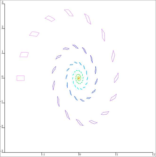
2D : Pendulum

Say that we want to integrate the state of the pendulum starting from the an initial box. It is defined by

\[\begin{split}\dot{x}=\gamma(x) = \begin{pmatrix} x_2 \\ -5\cdot\sin (x_1) - 0.5\cdot x_2 \end{pmatrix}\end{split}\]

The corresponding code is:

capd::IMap vectorField_pend("par:l,g;var:t,w;fun:w,-sin(t)*5 - 0.5*w;");

VectorVar X_2d(1);
AnalyticFunction psi0_pend ({X_2d},{0.1*X_2d[0],0.1});
OctaSym id_2d ({1,2});
OctaSym s ({-2,1});

auto peibos_output_pend = PEIBOS(vectorField_pend, 20., 0.2, psi0_pend, {id_2d,s,s*s,s.invert()}, 0.02, {-M_PI/2.,0.});

auto m_v_par_2d_pend = reach_set(peibos_output_pend);

The result is

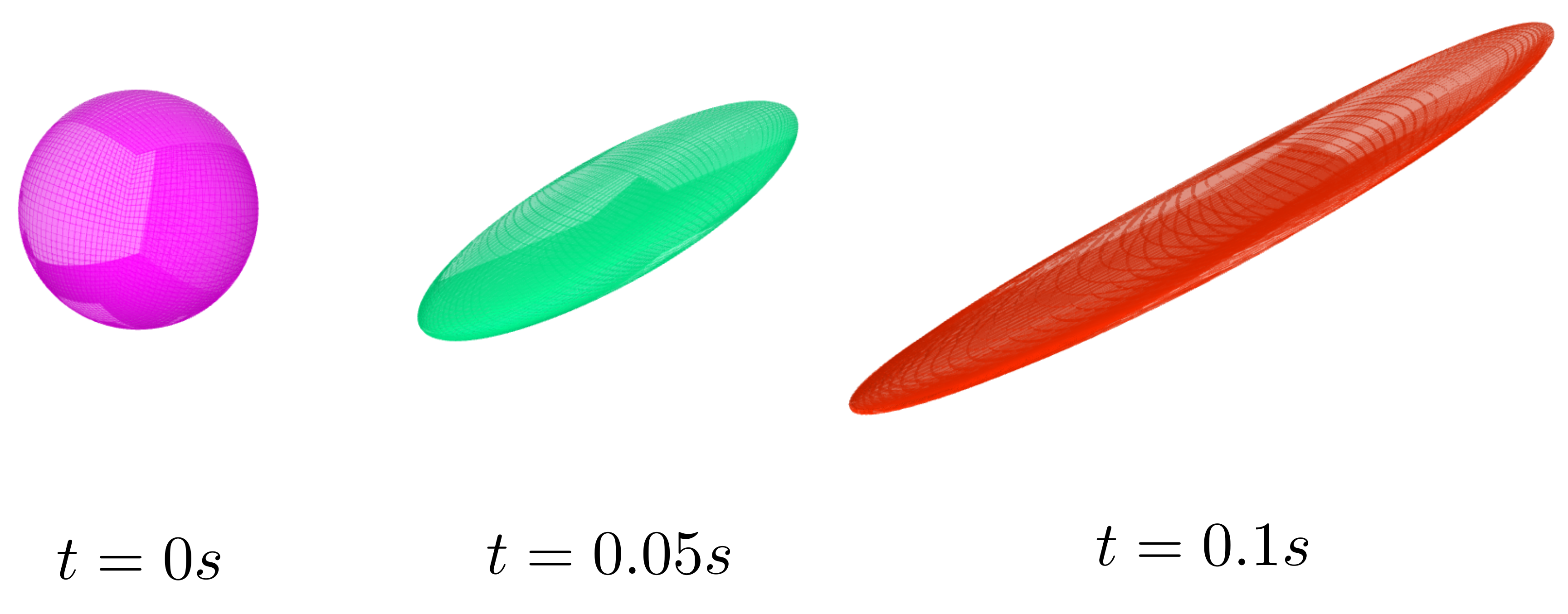
20 seconds of integration of the pendulum

3D : Lorenz system

Say that we want to integrate the state of the pendulum starting from the an initial sphere. It is defined by

\[\begin{split}\dot{x}=\gamma(x) = \begin{pmatrix} \sigma (x_2 - x_1) \\ x_1 (\rho - x_3) - x_2 \\ x_1 x_2 - \beta x_3 \end{pmatrix}\end{split}\]