Ellipsoid in n-dimensional space (matrix definition)

Main author: Morgan Louédec

Link to the Codac_ellipsoid_implementation

Definition of an Ellipsoid

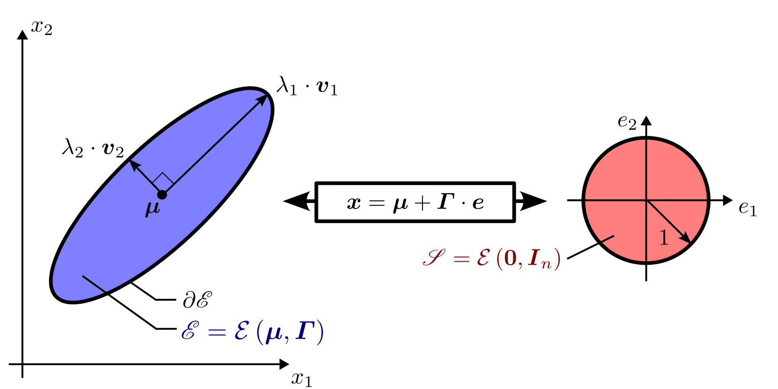
Figure 1 - Representation of a 2-dimensional ellipsoid \(\mathscr{E}\). The semi-axis of the ellipsoid are described by the eigenvalues and the eigenvectors of \(\boldsymbol{\Gamma}\).

An ellipsoid in \(n\)-dimensional space can be described by a unique midpoint \(\boldsymbol{\mu}\in\mathbb{R}^n\), a unique shape matrix \(\boldsymbol{\Gamma}\in S_n^+\) (real symmetric positive definite), and the quadratic form:

\[\mathcal{E}\left(\boldsymbol{\mu},\boldsymbol{\Gamma}\right) := \{\boldsymbol{x}\in\mathbb{R}^n | \left(\boldsymbol{x}-\boldsymbol{\mu}\right)^T \Gamma^{-2} \left(\boldsymbol{x}-\boldsymbol{\mu}\right) \leq 1\}.\]

When \(\boldsymbol{\mu}=\boldsymbol{0}\), the ellipsoid is said to be centred. The unitary eigenvectors \(\left\{\boldsymbol{v}_{1}, \boldsymbol{v}_{2},\cdots,\boldsymbol{v}_{n}\right\} \) of \(\boldsymbol{\varGamma}\) gives the direction of the semi-axis. The length of the semi-axis is given by the eigenvalues \(\left\{\lambda_{1}, \lambda_{2}, \cdots ,\lambda_{n}\right\} \) of \(\boldsymbol{\varGamma}\). The \(i^{\text{th}}\) semi-axis of \(\mathcal{E}\left(\boldsymbol{\mu},\boldsymbol{\varGamma}\right)\) is written \(\lambda_{i}\cdot\boldsymbol{v}_{i}\). The size of the ellipsoids can be evaluated as

\[\begin{align} \mathrm{size}\left(\mathcal{E}\left(\boldsymbol{\mu},\boldsymbol{\varGamma}\right)\right) = \det\left(\boldsymbol{\varGamma}\right) = \prod \limits_{i=1}^{n} \lambda_{i}. \end{align}\]

The surface of a two dimensional ellipsoid \(\mathscr{E}_2\) is given by \(S = \pi\cdot \textrm{size}\left(\mathscr{E}_2\right)\). The volume of a three dimensional ellipsoid \(\mathscr{E}_2\) is given by \(V = \frac{4\pi}{3}\cdot \textrm{size}\left(\mathscr{E}\right)\).

An ellipsoid can also be described by an affine transformation of the unit sphere:

\[\mathcal{E}\left(\boldsymbol{\mu},\boldsymbol{\Gamma}\right) = \boldsymbol{\mu} + \boldsymbol{\Gamma} \cdot \mathcal{E}\left(\boldsymbol{0},\boldsymbol{I_n}\right).\]

where \(\mathcal{E}\left(\boldsymbol{0},\boldsymbol{I_n}\right)\) is the unit sphere. More generally, an affine mapping of an ellipsoid \(\mathcal{E}\left(\boldsymbol{\mu}_1,\boldsymbol{\Gamma}_1\right)\) with a matrix \(\boldsymbol{A}\in\mathbb{R}^{n\times n}\) and a vector \(\boldsymbol{b}\in\mathbb{R}^n\) result in another ellipsoid:

\[\mathcal{E}\left(\boldsymbol{\mu}_2,\boldsymbol{\Gamma}_2\right) = \boldsymbol{A} \cdot \mathcal{E}\left(\boldsymbol{\mu}_1,\boldsymbol{\Gamma}_1\right) + \boldsymbol{b},\]

with \(\boldsymbol{\mu}_2 = \boldsymbol{A} \cdot \boldsymbol{\mu}_1 + \boldsymbol{b}\) and \(\boldsymbol{\Gamma}_2 = \left(\boldsymbol{A}\boldsymbol{\varGamma}_1^{2}\boldsymbol{A}^{T}\right)^{\frac{1}{2}}\).

Inclusion of ellipsoids

For two ellipsoids \(\mathscr{E}_{1}=\mathcal{E}\left(\boldsymbol{\mu}_1,\boldsymbol{\Gamma}_1\right)\) and \(\mathscr{E}_{2}=\mathcal{E}\left(\boldsymbol{\mu}_1,\boldsymbol{\Gamma}_1\right)\), the inclusion and the strict inclusion are respectively denoted by the symbols \(\subseteq\) and \(\subset\) such that

\[\begin{align} \left(\mathscr{E}_{1}\subset\mathscr{E}_{2}\right) & \Leftrightarrow\left(\mathscr{E}_{1}\subseteq\mathscr{E}_{2}\,\,\text{and} \,\,\mathscr{E}_{1}\cap\partial\mathscr{E}_{2}=\emptyset\right)\label{eq:inclusion_definition}. \end{align}\]

If two ellipsoids have the same midpoint (\(\boldsymbol{\mu}_1 = \boldsymbol{\mu}_2\)), their mutual inclusion can be verified using their shape matrices:

\[\begin{split}\begin{align} \left(\mathscr{E}_{1}\subseteq\mathscr{E}_{2}\right) & \Leftrightarrow\left(\boldsymbol{\varGamma}_{1}^{-2}-\boldsymbol{\varGamma}_{2}^{-2}\succeq0\right),\\ \left(\mathscr{E}_{1}\subset\mathscr{E}_{2}\right) & \Leftrightarrow\left(\boldsymbol{\varGamma}_{1}^{-2}-\boldsymbol{\varGamma}_{2}^{-2}\succ0\right). \end{align}\end{split}\]

Orthogonal projection of ellipsoids on affine space [1,Section 13]

Consider the orthogonal matrix \(\boldsymbol{T}=\left[\begin{array}{cc} \boldsymbol{t}_{1} & \boldsymbol{t}_{2}\end{array}\right]\in\mathbb{R}^{n\times2}\) and the plane

\[\begin{align} \mathcal{A}_{t_{1},t_{2}} & :=\left\{ \boldsymbol{x}\in\mathbb{R}^{n}|\exists\boldsymbol{t}\in\mathbb{R}^{2},\boldsymbol{x}=\boldsymbol{T}\cdot\boldsymbol{t}\right\}. \end{align}\]

The projection of an ellipsoid \(\mathscr{E}\) of \(\mathbb{R}^{n}\) onto the affine space \(\mathcal{A}_{i,j}\) results in the ellipsoid

\[\begin{split}\begin{align} \boldsymbol{p}_{\mathcal{A}_{t_{1},t_{2}}}\left(\mathscr{E}\right) & =\left(\boldsymbol{T}\boldsymbol{T}^{T}\right)\cdot\mathscr{E},\nonumber \\ & =\mathcal{\mathcal{E}}\left(\boldsymbol{T}\boldsymbol{T}^{T}\boldsymbol{\mu},\left(\boldsymbol{T}\boldsymbol{T}^T\boldsymbol{\varGamma}^{2}\boldsymbol{T}\boldsymbol{T}^{T}\right)^{\frac{1}{2}}\right) \end{align}\end{split}\]

with \(\left(\boldsymbol{\mu},\boldsymbol{\varGamma}\right)=\mathcal{E}^{-1}\left(\mathscr{E}\right)\) and such that \(\boldsymbol{p}_{\mathcal{A}_{t_{1},t_{2}}}\left(\mathscr{E}\right)\subset\mathcal{A}\). Then, with a change of variable \(\boldsymbol{y}=\boldsymbol{T}^{T}\cdot\boldsymbol{x}\), one can display the projected ellipsoid \(\boldsymbol{p}_{\mathcal{A}_{t_{1},t_{2}}}\left(\mathscr{E}\right)\) in the frame \(\left(\boldsymbol{0},\boldsymbol{t}_{1},\boldsymbol{t}_{2}\right)\), as illustrated by Figure 2.

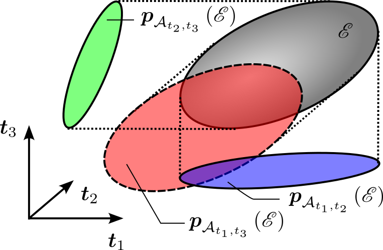
Figure 2 - A \(3\)-dimensional ellipsoid can be displayed with three \(2\)-dimensional orthogonal projections with three orthogonal vectors \(\boldsymbol{t}_{1}\), \(\boldsymbol{t}_{2}\) and \(\boldsymbol{t}_{3}\).

References

• [1] Stephen B Pope. Algorithms for Ellipsoids. page 49, 2008