[new] Lesson D: SLAM
Main authors: Simon Rohou
We propose to apply interval tools for solving a classical state estimation problem of Simultaneous Localization And Mapping (SLAM).
A tank robot \(\mathcal{R}\), described by the state vector \(\mathbf{x}\in\mathbb{R}^3\) depicting its position \((x_1,x_2)^\intercal\) and its heading \(x_3\), is evolving among a set of landmarks \(\mathbf{b}^k\in\mathbb{R}^2\) with a constant speed \(v=10\). It is equipped with a compass for measuring its heading \(x_3\) with some uncertainties.
Formalism
We are addressing the following state estimation problem:
The evolution of the state is given by:
and the system input \(u\) (rotation rate) is expressed as:
The observation function \(g\) is the distance function between a position \((x_1,x_2)^\intercal\) and a landmark \((b_1^k,b_2^k)^\intercal\).
Exercise
D.1. Update your current version of Codac:
pip install codac --upgrade --pre
# Option --pre has to be set because Codac v2 is only available in pre-release
The following instructions are given in Python, but feel free to use C++ or Matlab if you prefer.
Simulation
The following code provides a simulation of the actual but unknown trajectory \(\mathbf{x}^*(\cdot)\), without uncertainties. This code can be used as a starting point of your project.
from codac import *
import random
import numpy as np

dt = 0.02 # temporal discretization
t0tf = Interval(0,15) # [t0,tf]

# System input
t = ScalarVar()
u = AnalyticTraj(AnalyticFunction([t],3*(sin(t)^2)+t/100), t0tf).sampled(dt)

truth_heading = u.primitive()
truth_px = (cos(truth_heading)*10.).primitive()
truth_py = (sin(truth_heading)*10.).primitive()

# Actual state trajectory
# Note that this trajectory is unknown of the resolution
var_s1,var_s2,var_s3 = ScalarVar(),ScalarVar(),ScalarVar()
f_concat = AnalyticFunction([var_s1,var_s2,var_s3], [var_s1,var_s2,var_s3])
truth_x = f_concat.traj_eval(truth_px,truth_py,truth_heading)

DefaultFigure.draw_trajectory(truth_x)
Using VIBes, you should visualize these states:
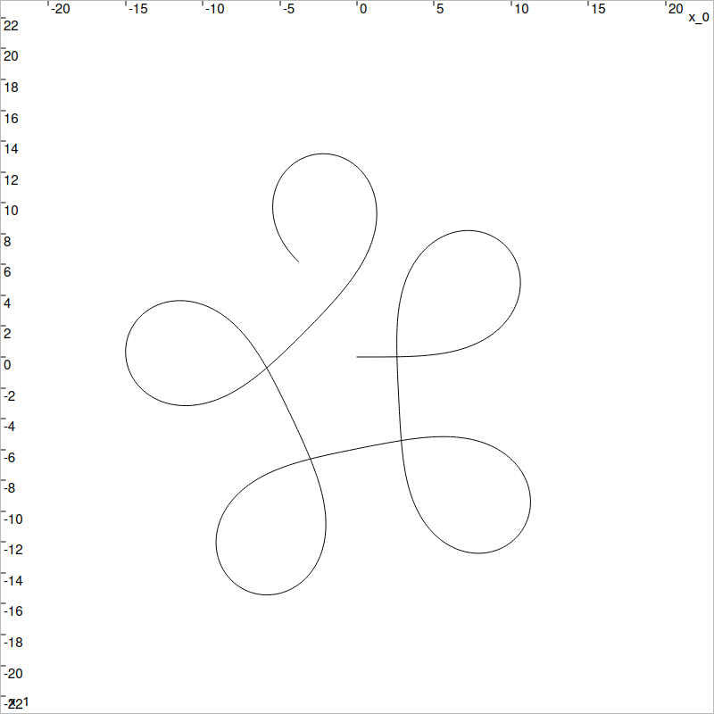
Unknown actual trajectory, to be estimated.
Deadreckoning
The robot knows its initial state: \(\mathbf{x}(0)=(0,0,0)^\intercal\). Deadreckoning consists in estimating the following positions of the robot without exteroceptive measurements (i.e. without distances from the landmarks). In this section, we will compute the set of feasible positions of \(\mathcal{R}\), considering only heading measurements and the evolution function \(\mathbf{f}\).
Exercise
D.2. Domains. The set of feasible positions along time is a tube (interval of trajectories). We create a tube \([\mathbf{x}](t)\) using:
tdomain = create_tdomain(t0tf, dt)
x = SlicedTube(tdomain, IntervalVector(3))
where tdomain is the temporal discretization over \([t_0,t_f]\),
and dt is the discretization parameter. Here, x is a 3d tube.
At this point, \(\forall t\in[t_0,t_f],~ [\mathbf{x}](t)=[-\infty,\infty]^3\): the states are completely unknown.
This can be verified, for instance at \(t=0\), with:
print(x(0.))
Exercise
D.3. Heading measurements. In practice, the headings \(x_3(t)\) are measured with some uncertainties known to be bounded in \([-0.03,0.03]\). We set these bounded measurements in the last component of the tube vector \([\mathbf{x}](t)\) as:
x = tube_cart_prod(
  SlicedTube(tdomain, IntervalVector(2)),
  # Heading measurement with bounded uncertainties:
  SlicedTube(tdomain, truth_heading).inflate(0.03)
)
Exercise
D.4. Initial condition. The initial state \(\mathbf{x}(0)\) (position and heading) is known, which can be implemented in the tube with:
x.set([0,0,0], 0.) # setting a vector value at t=0
print(x(0.))
Now that a domain (a tube) has been defined for enclosing the estimates together with their uncertainties, it remains to define contractors for narrowing their bounds.
In deadreckoning, only Eq. (2) is considered: \(\dot{\mathbf{x}}(t)=\mathbf{f}(\mathbf{x}(t))\). This can be processed with two contractors, one for dealing with \(\mathbf{v}(t)=\mathbf{f}(\mathbf{x}(t))\), and one for \(\dot{\mathbf{x}}(t)=\mathbf{v}(t)\).
The new tube \([\mathbf{v}](t)\) will enclose the feasible derivatives of the possible states in \([\mathbf{x}](t)\).
Exercise
D.5. Contractors. As for \([\mathbf{x}](t)\), create another 3d SlicedTube for
\([\mathbf{v}](t)\), called v.
Then, create a contractor for \(\mathbf{v}(t)=\mathbf{f}(\mathbf{x}(t))\). The associated constraint is expressed as an implicit form \(\mathbf{f}(\mathbf{x}(t),\mathbf{v}(t))=\mathbf{0}\).
var_x,var_v = VectorVar(3),VectorVar(3)
f_evol = AnalyticFunction([var_x,var_v], [
    var_v[0]-10*cos(var_x[2]),
    var_v[1]-10*sin(var_x[2]),
  ])

ctc_f = CtcInverse(f_evol, [0,0]) # [0,0] stands for the implicit form f(..)=0
Create a contractor for \(\dot{\mathbf{x}}(t)=\mathbf{v}(t)\):
ctc_deriv = CtcDeriv()
We recall that contractors are algorithms for reducing sets of feasible values (intervals, boxes, tubes..).
Exercise
D.6. Deadreckoning estimation. At this point, you can implemented an algorithm for deadreckoning, by calling the previously defined contractors.
ctc_f.contract_tube(x,v)
ctc_deriv.contract(x,v)
Exercise
D.7. Display. Eventually, the contracted tube \([\mathbf{x}](t)\) can be displayed with:
DefaultFigure.draw_tube(x, [Color.light_gray(),Color.light_gray()])
DefaultFigure.draw_trajectory(truth_x)
You should obtain the following result:
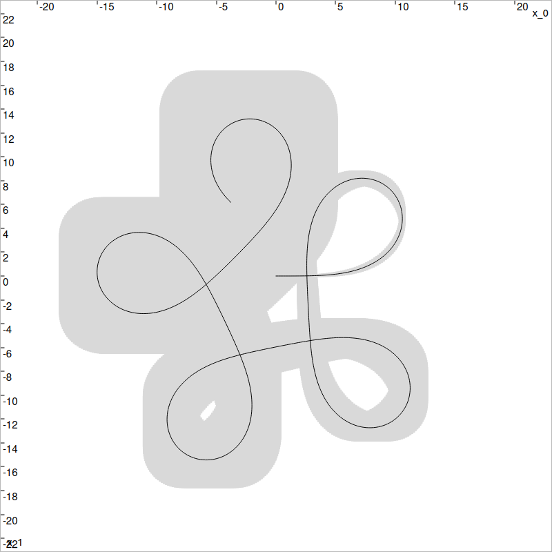
In gray: tube \([\mathbf{x}](t)\) enclosing the estimated trajectories of the robot. The actual but unknown trajectory is depicted in black. With interval methods, the computations are guaranteed: the actual trajectory cannot be outside the tube. However, the tube may be large in case of poor localization, as it is the case up to now without state observations.
Range-only localization
The obtained tube grows with time, illustrating a significant drift of the robot. We now rely on distances measured from known landmarks for reducing this drift. This amounts to a non-linear state estimation problem: function \(g\) of System (1) is a distance function. Non-linearities can be difficult to solve with conventional methods.
Exercise
D.8. Landmarks. Define five landmarks with:
b = [(6,12),(-2,-5),(-3,20),(3,4),(-10,0)]
Exercise
D.9. Range observations. In a loop, for each \(t_i\in\{0,1,\dots,15\}\), compute the distance measured from a random landmark:
Y = []
for ti in np.arange(0,15):
  k = random.randint(0,len(b)-1) # a random landmark is perceived
  d = sqrt(sqr(truth_x(ti)[0]-b[k][0])+sqr(truth_x(ti)[1]-b[k][1]))
  Y.append([k,ti,d])
Exercise
D.10. Measurement uncertainty. The measurements come with some errors (not computed here) that are known to be bounded within \([-0.03,0.03]\). We use intervals for enclosing the observations:
...
  d += Interval(-0.03,0.03)
  # or equivalently: d.inflate(3e-2)
As in the previous lessons, a fixpoint function can be used to manage the contractors automatically.
In another for loop, we will combine contractors using a fixpoint method, in order to improve the localisation of the robot.
Exercise
D.11. Observation contractors. The state observations are added to the set of constraints by means of a new distance contractor linking the state to the position of a landmark:
var_b = VectorVar(2)
var_d = ScalarVar()
f_dist = AnalyticFunction([var_x,var_b,var_d], sqrt(sqr(var_x[0]-var_b[0])+sqr(var_x[1]-var_b[1]))-var_d)
ctc_dist = CtcInverse(f_dist, 0) # also expressed in a implicit form g(x,b,d)=0
Exercise
D.12. Range-only localization. The network of contractors that you can implement is now the following:
def contractors_list(x,v):
  ctc_deriv.contract(x,v)
  ctc_f.contract_tube(x,v)
  for yi in Y: # for each range-only measurement
    ti = yi[1]
    pi = x(ti)
    bi = IntervalVector(b[yi[0]])
    di = yi[2]
    pi,bi,di = ctc_dist.contract(pi,bi,di)
    x.set(pi, ti)
  return x,v

x,v = fixpoint(contractors_list, x,v)
Exercise
D.13. Reveal the contracted tube.
DefaultFigure.draw_tube(x, ColorMap.blue_tube())
DefaultFigure.draw_trajectory(truth_x)
DefaultFigure.draw_tank(truth_x(t0tf.ub()), 1., [Color.dark_gray(),Color.yellow()])
You should obtain the following result:
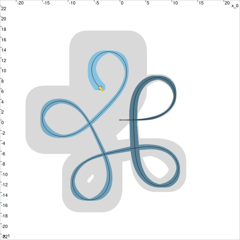
In gray: the former tube without state observations. In blue, the new contracted tube, considering distance measurements from the landmarks.
Exercise
Try to remove the condition set in Exercise D.4., and zoom towards the initial position.
Challenge: Simultaneous Localization and Mapping (SLAM)
Exercise
D.15. Range only SLAM.
Adapt the script in order to deal with a SLAM problem, in which the positions of the landmarks are priorly unknown, but then estimated together with the positions of the robot.
Note that in SLAM, the initial condition set in Exercise D.4. is mandatory.