Lesson C: Dynamic localization

We now propose to extend the previous lesson to the dynamic case, i.e. with a mobile robot evolving in the middle of a field of indistinguishable landmarks.

Formalism

The state is now with a fourth dimension for depicting the velocity of the robot. We are now addressing the following state estimation problem, with \(\mathbf{x}\in\mathbb{R}^4\):

\[\begin{split}\left\{ \begin{array}{lll} \dot{\mathbf{x}}(t)=\mathbf{f}\big(\mathbf{x}(t),\mathbf{u}(t)\big) & & \textrm{(evolution equation)}\\ \mathbf{y}_i=\mathbf{g}\big(\mathbf{x}(t_i),\mathbf{m}_i\big) & & \textrm{(observation equation)}\\ \mathbf{m}_i\in\mathbb{M} & & \textrm{(association constraint)} \end{array}\right.\end{split}\]

The asynchronous measurements \(\mathbf{y}_i\in\mathbb{R}^2\) are obtained for each time instants \(t_i\in[t_0,t_f]\). In this lesson, because the times \(t_i\) are supposed to be exactly known, these constraints will be dealt with as restrictions on tubes. Note that in case of time uncertainties, \(t_i\in[t_i]\), we should have used a specific contractor for reliability purposes.

The evolution function \(\mathbf{f}\) depicts the evolution of the state with respect to some input vector \(\mathbf{u}\):

\[\begin{split}\dot{\mathbf{x}}=\mathbf{f}(\mathbf{x},\mathbf{u})=\left( \begin{array}{c} x_4\cos(x_3) \\ x_4\sin(x_3) \\ u_1 \\ u_2 \end{array}\right),\end{split}\]

where \((x_1,x_2)^\intercal\) is the 2d position of the robot, \(x_3\) its heading and \(x_4\) its velocity.

The input \(\mathbf{u}(\cdot)\) is unknown, but we assume that we have continuous measurements for the headings \(x_3(\cdot)\) and the speeds \(x_4(\cdot)\), with some bounded uncertainties defined by intervals \([e_3]=[-0.02,0.02]\), \([e_4]=[-0.02,0.02]\).

Lastly, we do not have any knowledge about the initial position of the robot.

Decomposition

Exercise

C.1. In the first lesson, we wrote a decomposition of the static range and bearing problem. We extend this decomposition to deal with the dynamical case. This will make appear new intermediate variables. We propose the following decomposition:

• external trajectory variables: \(\mathbf{x}(\cdot)\in[t_0,t_f]\to\mathbb{R}^4\)

• intermediate trajectory variables: \(\mathbf{v}(\cdot)\in[t_0,t_f]\to\mathbb{R}^4\)

• external static variables (for each observation): \(\mathbf{y}_i\in\mathbb{R}^2\), \(\mathbf{m}_i\in\mathbb{R}^2\)

• intermediate static variables (for each observation): \(a_i\in\mathbb{R}\), \(\mathbf{d}_i\in\mathbb{R}^2\)

• constraints:

\[\begin{split}\left\{ \begin{array}{rl} (i) & \mathcal{L}_\textrm{polar}\big(d_1,d_2,y_{i,1},a_i\big):~~~\mathbf{d}_i=y_{i,1}\cdot\left(\hspace{-0.1cm}\begin{array}{c} ~\cos(a_i)~\\ ~\sin(a_i)~ \end{array}\hspace{-0.1cm}\right)\\ (ii) & d_{i,1} = m_{i,1}-x_1(t_i) \\ (iii) & d_{i,2} = m_{i,2}-x_2(t_i) \\ (iv) & a_i=x_3(t_i)+y_{i,2} \\ \textcolor{blue}{(v)} & \textcolor{blue}{\mathbf{v}(\cdot)=\mathbf{f}\left(\mathbf{x}(\cdot)\right)} \\ \textcolor{blue}{(vi)} & \textcolor{blue}{\dot{\mathbf{x}}(\cdot)=\mathbf{v}(\cdot)} \end{array}\right.\end{split}\]

The blue constraints are related to the dynamical case.

The input \(\mathbf{u}(\cdot)\) is not involved in this decomposition, as the velocity and speed are measured.

Initialization

Before going into a set-membership state estimation, we set up a simulation environment to test different random situations.

Exercise

(reuse your code from the previous lesson)

C.2. Using the following code, generate a set of randomly positionned landmarks:

PythonC++

srand() # initialize the random seed (from C++)
N = 50 # number of landmarks
X = IntervalVector([[-40,40],[-40,40]]) # landmarks distribution zone

M = [] # creating the landmarks
for i in range (0,N):
  M.append(IntervalVector(X.rand()).inflate(0.2))

fig = Figure2D("Robot simulation", GraphicOutput.VIBES)
fig.set_axes(
  axis(0, X[0].inflate(10), "x_1"),
  axis(1, X[1].inflate(10), "x_2")
).auto_scale()

for mi in M: # displaying the landmarks
  fig.draw_box(mi, [Color.dark_green(),Color.green()])

C.3. Now, we simulate a mobile robot moving in the middle of the field of landmarks. The trajectory is defined by a set of random waypoints. The class RobotSimulator is used to simplify the simulation:

PythonC++

wpts = [] # creating random waypoints for simulating the robot trajectory
X = IntervalVector([[-35,35],[-35,35]]) # robot evolution zone
for i in range (0,5): # 5 waypoints
  wpts.append(X.rand())

s = RobotSimulator()
s.w_max = 0.2 # maximum turning speed
u = SampledVectorTraj() # the simulator will return the inputs (not used)
x_truth = s.simulate(
  [0,0,0,0], # initial state (will be supposed unknown)
  1e-2, # simulation time step
  wpts, u)

C.4. We update the observation function g of the previous lessons for the dynamical case. To ease the code, the returned observation vector will contain the observation time \(t_i\).

PythonC++

def g(t,x,M):

  obs = [] # several landmarks can be seen at some ti
  scope_range = Interval(0,10)
  scope_angle = Interval(-PI/4,PI/4)

  for mi in M:
  
    r = sqrt(sqr(mi[0]-x[0]) + sqr(mi[1]-x[1]))
    a = atan2(mi[1]-x[1], mi[0]-x[0]) - x[2]

    # If the landmark is seen by the robot:
    if scope_range.is_superset(r) and scope_angle.is_superset(a):
      obs.append(IntervalVector([t,r,a]))

  return obs

C.5. Finally, we run the simulation for generating and drawing the observation vectors. obs contains all the observation vectors.

PythonC++

prev_t = 0.
time_between_obs = 3.
obs = []

t = x_truth.tdomain().lb()
while t < x_truth.tdomain().ub():

  if t-prev_t > time_between_obs:
    obs_ti = g(t,x_truth(t),M) # computing the observation vector

    for yi in obs_ti:
      prev_t = yi[0].mid()
      fig.draw_pie(x_truth(t).subvector(0,1), yi[1]|0., yi[2]+x_truth(t)[2], Color.light_gray())
      fig.draw_pie(x_truth(t).subvector(0,1), yi[1],    yi[2]+x_truth(t)[2], Color.red())

    obs.extend(obs_ti)

  t += 1e-2

State estimation with constraint programming

Exercise

C.6. Domains. We first create the tube \([\mathbf{x}](\cdot)\) that will contain the set of feasible state trajectories. In Codac, a tube is built as a list of slices, the temporal sampling of which is defined as a temporal domain (TDomain) that must be created beforehand. Several tubes can stand on a same TDomain. Then, the tube x is created according to the problem: we do not know its first two components for the positions, but the headings and velocities are known with some bounded errors. We define a function h for this purpose of initialization.

PythonC++

_x = VectorVar(4)
h = AnalyticFunction([_x],
  [
    # Positions are not known..
    Interval(-oo,oo), 
    Interval(-oo,oo),
    # But headings (x3) and velocities (x4) are bounded..
    _x[2] + 2e-2*Interval(-1,1),
    _x[3] + 2e-2*Interval(-1,1)
  ])

tdomain = create_tdomain(x_truth.tdomain(), 5e-2, True)
# The tube x is created from the interval evaluation of the actual trajectory
x = h.tube_eval(SlicedTube(tdomain,x_truth))
# The tube v is created as a four-dimensional tube of infinite values
v = SlicedTube(tdomain, IntervalVector([[-oo,oo],[-oo,oo],[-oo,oo],[-oo,oo]]))

In the above code, the intermediate variable \(\mathbf{v}(\cdot)\) has also its own domain v. It is initialized to \([-\infty,\infty]\) for each dimension.

C.7. Contractors. We re-use the contractors of the previous lesson: \(\mathcal{C}_+\), \(\mathcal{C}_-\), \(\mathcal{C}_{\mathrm{polar}}\), \(\mathcal{C}_{\mathbb{M}}\). It remains to create the contractors related to the tubes (blue constraints \((v)\) and \((vi)\)). One of them is already available in the catalog of contractors of the library: \(\mathcal{C}_{\mathrm{deriv}}\left([\mathbf{x}](\cdot),[\mathbf{v}](\cdot)\right)\) for the constraint \(\dot{\mathbf{x}}(\cdot)=\mathbf{v}(\cdot)\). The other \(\mathcal{C}_\mathbf{f}\) contractor can be defined as previously, according to the evolution function.

PythonC++

ctc_deriv = CtcDeriv()

_x, _v = VectorVar(4), VectorVar(4)
f = AnalyticFunction([_x,_v],
  [
    _v[0]-_x[3]*cos(_x[2]),
    _v[1]-_x[3]*sin(_x[2])
  ])

ctc_f = CtcInverse(f, [0,0])
# + other contractors from previous lessons:
# ctc_plus, ctc_minus, ctc_polar, ctc_constell

C.8. Fixpoint resolution. Finally, the propagation loops need to be updated to incorporate the dynamic constraints. Note that the contractors \(\mathcal{C}_\mathbf{f}\) and \(\mathcal{C}_{\mathrm{deriv}}\) apply to the whole tubes \([\mathbf{x}](\cdot)\) and \([\mathbf{v}](\cdot)\). Furthermore, the class CtcInverse can contract tubes using the .contract_tube(..) method, exactly as we would do for boxes. Finally, a restriction on a tube (i.e. setting a value to a slice) can be done using the .set(y,t) method, for setting the interval vector value y at time t.

PythonC++

def ctc_one_obs(xi,yi,mi,ai,si):

  mi,xi,si = ctc_minus.contract(mi,xi,si)
  xi[2],yi[2],ai = ctc_plus.contract(xi[2],yi[2],ai)
  si[0],si[1],yi[1],ai = ctc_polar.contract(si[0],si[1],yi[1],ai)
  mi = ctc_constell.contract(mi)

  return xi,yi,mi,ai,si

def ctc_all_obs(x):
  global v

  for yi in obs:
    xi = x(yi[0]) # evalution of the tube at time ti=yi[0]
    ai = Interval()
    si = IntervalVector(2)
    mi = IntervalVector(2)
    xi,yi,mi,ai,si = fixpoint(ctc_one_obs, xi,yi,mi,ai,si)
    x.set(xi,yi[0]) # restriction on the tube x at time ti=yi[0]

  x,v = ctc_f.contract_tube(x,v)
  x = ctc_deriv.contract(x,v)

  return x

x = fixpoint(ctc_all_obs, x)

You should obtain a result similar to:

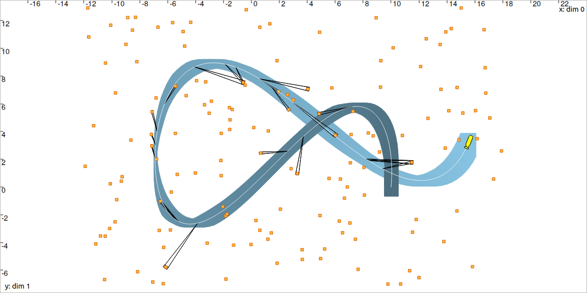
Localization by solving data association: the state trajectory \(\mathbf{x}(\cdot)\) (in white) has been estimated (in blue) together with the identification of the perceived landmarks.

Why is this problem of localization and data association difficult?

1. We do not know the initial condition of the system. Contrary to other approaches, this solver made of contractors does not require some initial vector \(\mathbf{x}_0\) to start the estimation. Information is taken into account from anytime in \([t_0,t_f]\).

2. The constraints are heterogeneous: some of them are said continuous (they act on continuous domains of values, for instance intervals). Other are discrete (for instance, the identity of landmarks, estimated among a discrete set of \(n\) possible values). And finally, some constraints come from differential equations (for instance for depicting the robot evolution). In this solver, we show that any kind of constraint can be combined, without going into a complex resolution algorithm.

3. We do not have to linearize, and thus there is no approximation made here. This means that the equations are directly set in the solver, without transformation. Furthermore, the results are reliable: we can guarantee that the actual trajectory is inside the tube \([\mathbf{x}](\cdot)\).