Parallelepiped inclusion function
Main author: Maël Godard
Use case
Consider a function \(\mathbf{f}:\mathbb{R}^n\to\mathbb{R}^m\). In the case where \(0<n<m\), a parallelepiped inclusion function is available in the library.
A parallelepiped inclusion function of \(\mathbf{f}\) is noted \(\langle\mathbf{f}\rangle\). For a \(n\)-dimensional box \([\mathbf{x}]\), \(\langle\mathbf{f}\rangle([\mathbf{x}])\) is a parallelepiped which enclose \(\mathbf{f}([\mathbf{x}])\).
Note that this inclusion function also works with thick functions.
Examples
\(\mathbb{R}^1\to\mathbb{R}^2\)
Define the parabolic function \(\mathbf{f}:\mathbb{R}\to\mathbb{R}^2\) such that
It can be defined in Codac as follows:
X_2d = ScalarVar()
f_2d = AnalyticFunction([X_2d], [X_2d,sqr(X_2d)])
ScalarVar X_2d;
AnalyticFunction f_2d({X_2d},{X_2d,sqr(X_2d)});
X_2d = ScalarVar();
f_2d = AnalyticFunction({X_2d},vec(X_2d,sqr(X_2d)));
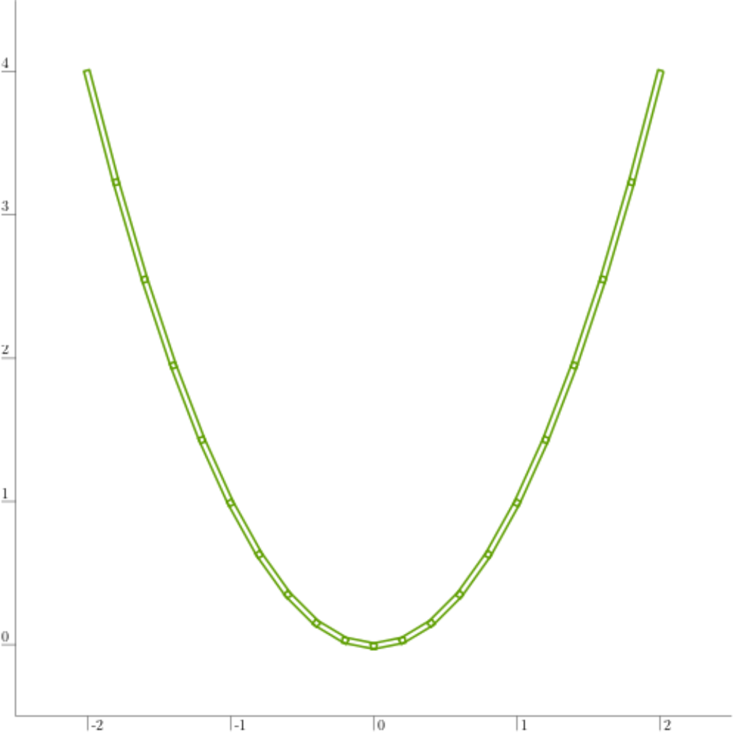
The performances of the parallelepiped inclusion function can be visualized as follows:
dx_2d = 0.2
x0_2d = -2.0

while x0_2d <= 2.0:
    X0_2d = Interval(x0_2d, x0_2d+dx_2d)
    p = f_2d.parallelepiped_eval(X0_2d)
    DefaultFigure.draw_parallelepiped(p, Color.dark_green())

    x0_2d += dx_2d
double dx_2d = 0.2;
double x0_2d = -2.0;

while (x0_2d<2.0)
{
    Interval X0_2d(x0_2d, x0_2d+dx_2d);
    auto p = f_2d.parallelepiped_eval(X0_2d);
    DefaultFigure::draw_parallelepiped(p, Color::dark_green());

    x0_2d+=dx_2d;
}
dx_2d = 0.2;
x0_2d = -2.0;

while x0_2d<2.0
    X0_2d = Interval(x0_2d,x0_2d+dx_2d);
    p = f_2d.parallelepiped_eval(X0_2d);
    DefaultFigure().draw_parallelepiped(p,StyleProperties(Color().dark_green()));

    x0_2d = x0_2d + dx_2d;
end
The resulting plot is shown below. In green is the result of the evaluation using parallelepipeds.

\(\mathbb{R}^2\to\mathbb{R}^3\)
Define the parabolic function \(\mathbf{f}:\mathbb{R}^2\to\mathbb{R}^3\) such that
It can be defined in Codac as follows:
X_3d = VectorVar(2)
f_3d = AnalyticFunction([X_3d], [X_3d[0], X_3d[1], sqr(X_3d[0]) + sqr(X_3d[1])])
VectorVar X_3d(2);
AnalyticFunction f_3d({X_3d},{X_3d[0],X_3d[1],sqr(X_3d[0])+sqr(X_3d[1])});
X_3d = VectorVar(2);
f_3d = AnalyticFunction({X_3d},vec(X_3d(1),X_3d(2),sqr(X_3d(1))+sqr(X_3d(2))));
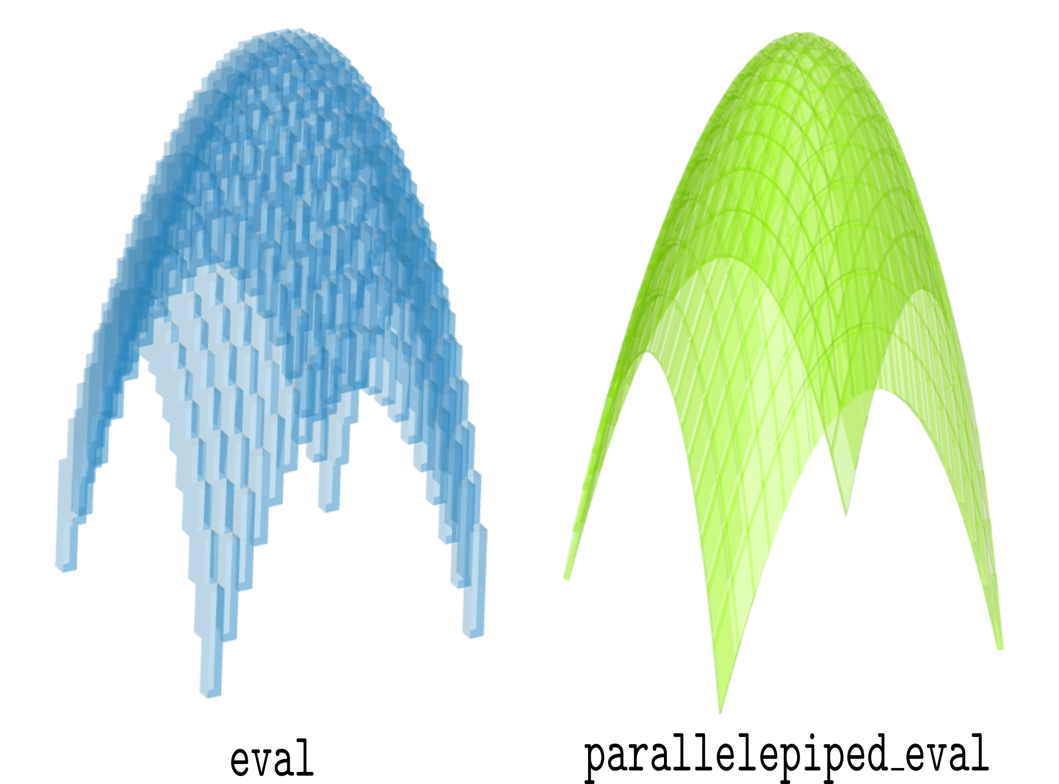
The performances of the parallelepiped inclusion function can be visualized as follows:
fig_3d = Figure3D("3D")
dx_3d = 0.2
x0_3d = -2.0

while x0_3d <= 2.0:
    X0_3d = Interval(x0_3d, x0_3d+dx_3d)
    y0_3d = -2.0

    while y0_3d <= 2.0:
        Y0_3d = Interval(y0_3d, y0_3d+dx_3d)
        b = f_3d.eval([X0_3d, Y0_3d])
        p = f_3d.parallelepiped_eval([X0_3d, Y0_3d])

        fig_3d.draw_box(b, StyleProperties(Color.blue(0.3), "box"))
        fig_3d.draw_parallelepiped(p, StyleProperties(Color.green(0.3), "parallelepiped"))

        y0_3d += dx_3d

    x0_3d += dx_3d
Figure3D fig_3d ("3D");

double dx_3d = 0.2;
double x0_3d = -2.0;

while (x0_3d<=2.0)
{
    Interval X0_3d(x0_3d, x0_3d+dx_3d);
    double y0_3d=-2.0;

    while (y0_3d<=2.0)
    {
        Interval Y0_3d(y0_3d, y0_3d+dx_3d);
        auto b = f_3d.eval(IntervalVector({X0_3d,Y0_3d}));
        auto p = f_3d.parallelepiped_eval(IntervalVector({X0_3d,Y0_3d}));

        fig_3d.draw_box(b, StyleProperties(Color::blue(0.3),"box"));
        fig_3d.draw_parallelepiped(p, StyleProperties(Color::green(0.3),"parallelepiped"));

        y0_3d+=dx_3d;
    }

    x0_3d+=dx_3d;
}
fig_3d = Figure3D("3D");
dx_3d = 0.2;
x0_3d = -2.0;

while x0_3d<=2.0
    X0_3d = Interval(x0_3d,x0_3d+dx_3d);
    y0_3d = -2.0;

    while y0_3d<=2.0
        Y0_3d = Interval(y0_3d,y0_3d+dx_3d);
        b = f_3d.eval(IntervalVector({X0_3d,Y0_3d}));
        p = f_3d.parallelepiped_eval(IntervalVector({X0_3d,Y0_3d}));

        fig_3d.draw_box(b, StyleProperties(Color().blue(0.3),"box"));
        fig_3d.draw_parallelepiped(p, StyleProperties(Color().green(0.3),"parallelepiped"));

        y0_3d = y0_3d + dx_3d;
    end

    x0_3d = x0_3d + dx_3d;
end
The resulting figure is shown below. On the left is the result of the interval evaluation of Codac (layer “box”) (see Evaluations). On the right is the evaluation using parallelepipeds (layer “parallelepiped”).

Thick function
Define the thick parabolic function \(\mathbf{f}:\mathbb{R}\to\mathbb{R}^2\) such that
It is called a thick function because the output of this function is always a box (here an interval) even when the input is a real number.
It can be defined in Codac as follows:
X_if = ScalarVar()
f_if = AnalyticFunction([X_if], [X_if,Interval(1.1,1.2)*sqr(X_if)])
ScalarVar X_if;
AnalyticFunction f_if({X_if},{X_if,Interval(1.1,1.2)*sqr(X_if)});
X_if = ScalarVar();
f_if = AnalyticFunction({X_if},vec(X_if,Interval(1.1,1.2)*sqr(X_if)));
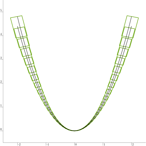
The thickness of the function can be visualized by plotting the lower and upper trajectories:
f_lb = AnalyticTraj(AnalyticFunction([X_if],1.1*sqr(X_if)),Interval(-2.0,2.0))
f_ub = AnalyticTraj(AnalyticFunction([X_if],1.2*sqr(X_if)),Interval(-2.0,2.0))

DefaultFigure.plot_trajectory(f_lb.sampled(0.01))
DefaultFigure.plot_trajectory(f_ub.sampled(0.01))
AnalyticTraj f_lb (AnalyticFunction({X_if},1.1*sqr(X_if)),Interval(-2.0,2.0));
AnalyticTraj f_ub (AnalyticFunction({X_if},1.2*sqr(X_if)),Interval(-2.0,2.0));

DefaultFigure::plot_trajectory(f_lb.sampled(0.01));
DefaultFigure::plot_trajectory(f_ub.sampled(0.01));
f_lb = AnalyticTraj(AnalyticFunction({X_if},1.1*sqr(X_if)),Interval(-2.0,2.0));
f_ub = AnalyticTraj(AnalyticFunction({X_if},1.2*sqr(X_if)),Interval(-2.0,2.0));

DefaultFigure().plot_trajectory(f_lb.sampled(0.01));
DefaultFigure().plot_trajectory(f_ub.sampled(0.01));
The performances of the parallelepiped inclusion function can then be visualized as follows:
dx_if = 0.1
x0_if = -2.0

while x0_if <= 2.0:
    X0_if = Interval(x0_if, x0_if+dx_if)
    p = f_if.parallelepiped_eval(X0_if)
    DefaultFigure.draw_parallelepiped(p, Color.dark_green())

    x0_if += dx_if
double dx_if = 0.1;
double x0_if = -2.0;

while (x0_if<=2.0)
{
    Interval X0_if(x0_if, x0_if+dx_if);
    auto p = f_if.parallelepiped_eval(X0_if);
    DefaultFigure::draw_parallelepiped(p, Color::dark_green());

    x0_if+=dx_if;
}
dx_if = 0.1;
x0_if = -2.0;

while x0_if<=2.0
    X0_if = Interval(x0_if,x0_if+dx_if);
    p = f_if.parallelepiped_eval(X0_if);
    DefaultFigure().draw_parallelepiped(p,StyleProperties(Color().dark_green()));

    x0_if = x0_if + dx_if;
end
The resulting plot is shown below. In green is the result of the evaluation using parallelepipeds, and in black are the lower and upper trajectories.
