PEIBOS

The PEIBOS tool provides a way to compute the Parallelepipedic Enclosure of the Image of the BOundary of a Set.

Let us consider an initial set $\mathbb{X}_0 \subset \mathbb{R}^n$ with its boundary $\partial \mathbb{X}_0$. Considering a function $\mathbf{f}:\mathbb{R}^n \to \mathbb{R}^p$, $n \leq p$, the PEIBOS tool allows to compute the set $\mathbf{Y}=\left\{ \mathbf{f}(\mathbf{x}) \mid \mathbf{x} \in \partial \mathbb{X}_0 \right\}$.

Gnomonic atlas

To handle the boundary of the initial set $\mathbb{X}_0$, the PEIBOS tool relies on a gnomonic atlas.

A gnomonic atlas of $\partial \mathbb{X}_0$ is composed of the inverse chat $\psi_0$ and a set of symmetries $\Sigma$ such that:

\[\partial \mathbb{X}_0 = \bigcup_{\sigma \in \Sigma} \sigma \circ \psi_0(\left[-1,1\right]^{m})\]

where $m$ is the dimension of the boundary $\partial \mathbb{X}_0$, $m < n$.

Example

Consider the case where $\mathbb{X}_0$ is the unit disk. Its boundary $\partial \mathbb{X}_0$ is the unit circle $\mathcal{S}^1$.

The image of $\left[-1,1\right]$ by the function

\[\begin{split}\begin{array}{ccc} \psi_{0} & : & \begin{array}{ccc} \mathbb{R} & \rightarrow & \mathbb{R}^{2}\\ x & \mapsto & \left( \begin{array}{c} \sin\left(x\cdot\frac{\pi}{4}\right)\\ \cos\left(x\cdot\frac{\pi}{4}\right) \end{array}\right) \end{array} \end{array}\end{split}\]

gives a quarter of $\mathcal{S}^1$. If we define $s$ the rotation of $\frac{\pi}{2}$, $\mathcal{S}^1$ can be covered by the gnomonic atlas $\left\{\psi_0,\left\{1,s,s^2,s^{-1}\right\}\right\}$ as shown below.

$Gnomonic atlas of :math:`\mathcal{S}^1`.$

Use

The PEIBOS function takes at least four arguments :

The studied analytic function.
The inverse chart for the gnomonic atlas (an analytic function).
The list of symmetries for the gnomonic atlas. Note that each symmetry is represented as a hyperoctahedral symmetry, see Octahedral symmetries.
A resolution $\epsilon$. The initial box $\left[-1,1\right]^m$ will initiallly be splitted in boxes with a diameter smaller than $\epsilon$.
Eventually an offset vector can be specified if the initial set is not centered around the origin.
Eventually a flag can be set to True to get the verbose.

For each of the small box $\left[\mathbf{x}\right]$, the PEIBOS algorithm uses the Parallelepiped inclusion function to enclose $\mathbf{f}\left(\sigma\left(\psi_0\left( \left[\mathbf{x}\right] \right)\right) + \text{offset}\right)$

It returns a vector of Parallelepiped. Their union is an outer approximation of $\mathbf{f}\left(\partial \mathbb{X}_0\right)$.

The full signature of the function is :

std::vector<Parallelepiped> codac2::PEIBOS(const AnalyticFunction<VectorType> &f, const AnalyticFunction<VectorType> &psi_0, const std::vector<OctaSym> &Sigma, double epsilon, const Vector &offset, bool verbose = false)

Compute a set of parallelepipeds enclosing $\mathbf{f}(\sigma(\psi_0([-1,1]^m)) + offset) $ for each symmetry $\sigma$ in the set of symmetries $\Sigma$. Note that $\left\{\psi_0,\Sigma\right\}$ form a gnomonic atlas.

Parameters:

f – The analytic function $\mathbf{f}:\mathbb{R}^n\rightarrow\mathbb{R}^p,p\geq n$
psi_0 – The transformation function $\psi_0:\mathbb{R}^m\rightarrow\mathbb{R}^n$ to construct the atlas
Sigma – The set of symmetry operators $\sigma$ to construct the atlas
epsilon – The maximum diameter of the boxes to split $[-1,1]^m$ before computing the parallelepiped inclusions
offset – The offset to add to $\sigma(\psi_0([-1,1]^m))$ (used to translate the initial manifold)
verbose – If true, print the time taken to compute the parallelepiped inclusions with other statistics

Returns:

A vector of Parallelepipeds enclosing $\mathbf{f}(\sigma(\psi_0([-1,1]^m))+ offset)$ for each symmetry $\sigma$ in the set of symmetries $\Sigma$.

Examples

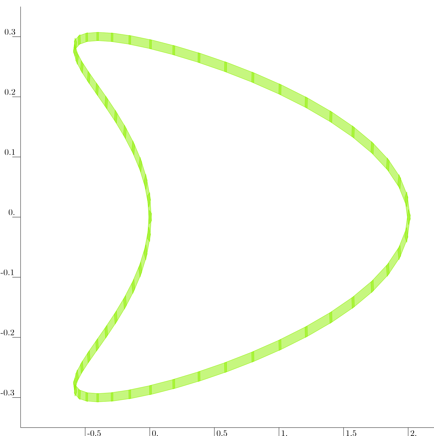
2D : Henon map

Say that we want to compute the image of the unit circle by the Henon map defined by

\[\begin{split}\mathbf{f}(\mathbf{x})=\left(\begin{array}{c} x_{2}+1-ax_{1}^{2}\\ bx_{1} \end{array}\right),a=1.4,b=0.3\end{split}\]

The corresponding code is:

# Definition of f
y_2d = VectorVar(2)
a,b = 1.4,0.3
f_2d = AnalyticFunction([y_2d],[y_2d[1]+1-a*sqr(y_2d[0]),b*y_2d[0]])

# Definition of the gnomonic atlas
X_2d = VectorVar(1)
psi0_2d = AnalyticFunction([X_2d],[sin(X_2d[0]*PI/4.),cos(X_2d[0]*PI/4.)])
id_2d = OctaSym([1, 2])
s = OctaSym([-2, 1])

# Call to PEIBOS
v_par_2d = PEIBOS(f_2d,psi0_2d,[id_2d,s,s*s,s.invert()],0.2)

// Definition of f
VectorVar y_2d(2);
double a = 1.4; double b = 0.3;
AnalyticFunction f_2d({y_2d},{y_2d[1]+1-a*sqr(y_2d[0]),b*y_2d[0]});

// Definition of the gnomonic atlas
VectorVar X_2d(1);
AnalyticFunction psi0_2d ({X_2d},{sin(X_2d[0]*PI/4.),cos(X_2d[0]*PI/4.)});
OctaSym id_2d ({1,2});
OctaSym s ({-2,1});

// Call to PEIBOS
auto v_par_2d = PEIBOS(f_2d, psi0_2d, {id_2d,s,s*s,s.invert()}, 0.2);

% Definition of f
y_2d=VectorVar(2);
a=1.4;
b=0.3;
f_2d = AnalyticFunction({y_2d},vec(y_2d(2)+1-a*sqr(y_2d(1)),b*y_2d(1)));

% Definition of the gnomonic atlas
X_2d = VectorVar(1);
psi0_2d = AnalyticFunction({X_2d},vec(sin(X_2d(1)*PI/4.),cos(X_2d(1)*PI/4.)));
id_2d = OctaSym(int64([1,2]));
s = OctaSym(int64([-2,1]));

% Call to PEIBOS
v_par_2d = PEIBOS(f_2d,psi0_2d,{id_2d,s,s*s,s.invert()},0.2);

The result is

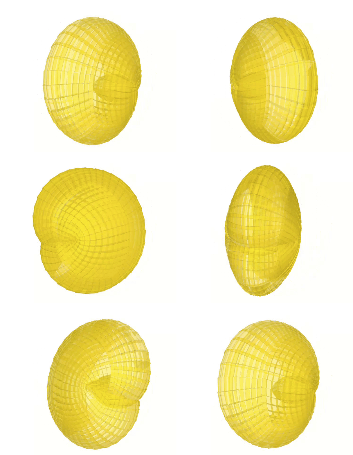
3D

Say that we want to compute the image of the unit sphere by the function defined by

\[\begin{split}\mathbf{f}(\mathbf{x})=\left(\begin{array}{c} x_{1}^{2}-x_{2}^{2}+x_{1}\\ 2x_{1}x_{2}+x_{2}\\ x_{3} \end{array}\right)\end{split}\]