The CtcDist contractor

Main author: Simon Rohou

class CtcDist : public codac2::Ctc<CtcDist, IntervalVector>

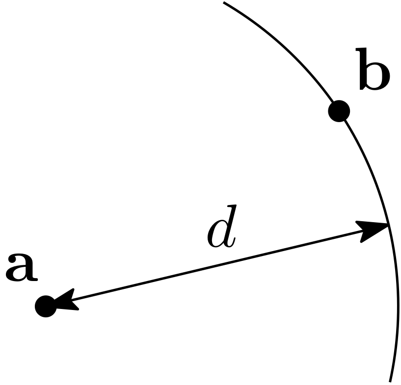
Implements the distance constraint on \(\mathbf{a}\in\mathbb{R}^2\), \(\mathbf{b}\in\mathbb{R}^2\) and \(d\in\mathbb{R}\) such that:

\[d^2=(a_1-b_1)^2+(a_2-b_2)^2. \]

The contractor can be applied either on a 5d box or on a set of five intervals.

This contractor is minimal.

Methods

void codac2::CtcDist::contract(IntervalVector &x) const

Applies \(\mathcal{C}_{\textrm{dist}}\big([\mathbf{x}]\big)\).

Parameters:: x – IntervalVector for \((a_1,a_2,b_1,b_2,d)^\intercal\)

x = IntervalVector([[2,5],[2,6],[0,0],[0,0],[1,3]])
c = CtcDist()
c.contract(x)
# x = [ [2, 2.23607] ; [2, 2.23607] ; <0, 0> ; <0, 0> ; [2.82842, 3] ]

IntervalVector x({{2,5},{2,6},{0,0},{0,0},{1,3}});
CtcDist c;
c.contract(x);
// x = [ [2, 2.23607] ; [2, 2.23607] ; <0, 0> ; <0, 0> ; [2.82842, 3] ]

void codac2::CtcDist::contract(Interval &a1, Interval &a2, Interval &b1, Interval &b2, Interval &d) const

Applies \(\mathcal{C}_{\textrm{dist}}\big([a_1],[a_2],[b_1],[b_2],[d]\big)\).

Parameters:

a1 – Interval for \(a_1\)
a2 – Interval for \(a_2\)
b1 – Interval for \(b_1\)
b2 – Interval for \(b_2\)
d – Interval for \(d\)

a1,a2,b1,b2,d = Interval(2,5),Interval(2,6),Interval(0),Interval(0),Interval(1,3)
c = CtcDist()
c.contract(a1,a2,b1,b2,d)
# a1 = [2, 2.23607] ; a2 = [2, 2.23607] ; b1 = <0, 0> ; b2 = <0, 0> ; d = [2.82842, 3]

Interval a1(2,5), a2(2,6), b1(0), b2(0), d(1,3);
CtcDist c;
c.contract(a1,a2,b1,b2,d);
// a1 = [2, 2.23607] ; a2 = [2, 2.23607] ; b1 = <0, 0> ; b2 = <0, 0> ; d = [2.82842, 3]

Example of use with a paver

A static robot located at \(\mathbf{x}=(0,0)^\intercal\) receives range-only (distance) signals from two landmarks located at \(\mathbf{b}^{(1)}=(1,2)^\intercal\) and \(\mathbf{b}^{(2)}=(3.6,2.4)^\intercal\). The observation equation \(y^{(i)}=g^{(i)}(\mathbf{x})\) is given by:

\[y^{(i)}=\sqrt{(x_1-b_1^{(i)})^2+(x_2-b_2^{(i)})^2},\]

where \(\mathbf{b}^{(i)}\) is the \(i\)-th landmark emitting range-only signals.

We assume that two distances are received from the landmarks. Considering bounded uncertainties, we state the actual observations are bounded as:

from \(\mathbf{b}^{(1)}\), \(y^{(1)}\in[2,2.4]\)
from \(\mathbf{b}^{(2)}\), \(y^{(2)}\in[4.1,4.5]\)

The \(\mathcal{C}_{\textrm{dist}}\) applies on 5d boxes but we are only interested in paving the \((x_1,x_2)\) space, so we will project the distance contractors associated with each landmark on \((x_1,x_2)\) using \(\mathcal{C}_{\textrm{proj}}\). The projection is restricted to the measurements and the position of the landmarks.

b1, b2 = Vector([1,2]), Vector([3.6,2.4])
y1, y2 = Interval(2,2.4), Interval(4.1,4.5)

c = CtcDist() # generic distance contractor
c1 = CtcProj(c, [0,1], cart_prod(b1,y1)) # projection involving data
c2 = CtcProj(c, [0,1], cart_prod(b2,y2))

Vector b1({1,2}), b2({3.6,2.4});
Interval y1(2,2.4), y2(4.1,4.5);

CtcDist c; // generic distance contractor
CtcProj c1(c, {0,1}, cart_prod(b1,y1)); // projection involving data
CtcProj c2(c, {0,1}, cart_prod(b2,y2));

Finally, we pave the intersection of each projected contractor.

draw_while_paving( # calling a paver algorithm for graphic output
  [[-3,5],[-2.5,5.5]], # initial 2d box
  c1 & c2, # intersection of the two projected contractors
  0.1 # paver precision
)

DefaultFigure.draw_ring(b1, y1)
DefaultFigure.draw_ring(b2, y2)
DefaultFigure.draw_circle([0,0], 0.1, [Color.red(),Color.red()])

draw_while_paving( // calling a paver algorithm for graphic output
  {{-3,5},{-2.5,5.5}}, // initial 2d box
  c1 & c2, // intersection of the two projected contractors
  0.1 // paver precision
);

DefaultFigure::draw_ring(b1, y1);
DefaultFigure::draw_ring(b2, y2);
DefaultFigure::draw_circle({0,0}, 0.1, {Color::red(),Color::red()});

We obtain the following approximation:

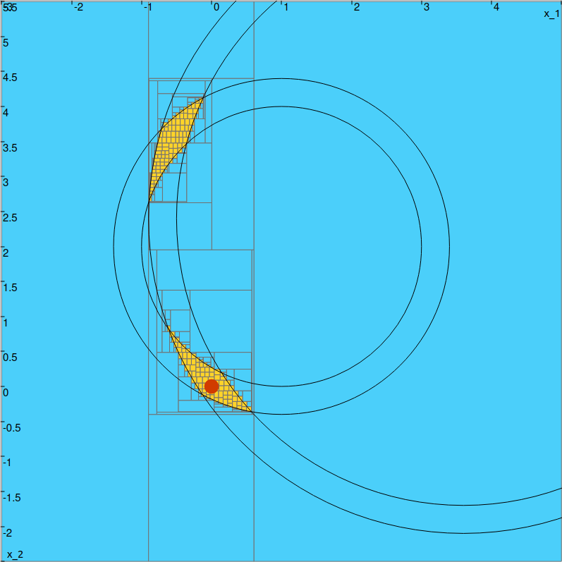
../../../_images/ctcdist_example.png — Outer approximation of the feasible position set.

Technical documentation

See the C++ API documentation of this class.