The CtcInverse contractor
Main author: Simon Rohou
Definition
Consider a function \(\mathbf{f}:\mathbb{R}^n\to \mathbb{R}^p\). The CtcInverse contractor allows one to handle constraints of the form \(\mathbf{f}(\mathbf{x})\in\mathbb{Y}\) by contracting input boxes \([\mathbf{x}]\in\mathbb{IR}^n\) while preserving all solutions consistent with the constraint set \(\mathbb{Y}\).
\(\mathbb{Y}\) is a constraint set on the codomain of \(\mathbf{f}\). Note that contractors are typically used when \(\mathbb{Y}\) is thin (e.g., equality constraints). For thick sets (inequalities), separators are often preferable to obtain both outer and inner approximations, and faster computations.
In Codac, \(\mathbb{Y}\) can be represented in two main ways:
Important
(i) Box representation
When \(\mathbb{Y}\) is given as a box \([\mathbf{y}]\), the constraint reads: \(\mathbf{f}(\mathbf{x}) \in [\mathbf{y}]\).
(ii) Contractor representation
More generally, \(\mathbb{Y}\) may be any output set representable by a contractor \(\mathcal{C}_{\mathbb{Y}}\): \(\mathbf{f}(\mathbf{x}) \in \mathcal{C}_{\mathbb{Y}}\).
In this case, \(\mathcal{C}_{\mathbb{Y}}\) is any contractor acting on boxes in \(\mathbb{R}^p\).
In the current version of Codac (v2), CtcInverse is the successor of the v1 CtcFunction contractor (renamed for clarity). It is also closely related to the CtcFwdBwd of the IBEX library.
Construction and basic usage
The typical workflow is:
Define analytic variables (scalar, vector, matrix) associated with the domain of the function.
Build an
AnalyticFunction.Instantiate
CtcInversewith a codomain constraint (a box \([\mathbf{y}]\) or a contractor \(\mathcal{C}_{\mathbb{Y}}\)).Contract an input box \([\mathbf{x}]\) or pave the contractor in the domain space.
Dealing with equalities and inequalities
Equalities are expressed with a degenerate interval (or box) in the codomain, e.g.:
\(f(x)=0\) is encoded as \(f(x)\in[0,0]\).
Inequalities are encoded by widening the codomain interval(s). For instance:
\(f(x)\leqslant 0\) is encoded as \(f(x)\in[-\infty,0]\).
In the case of inequalities, the use of the equivalent SepInverse separator should be preferred for efficiency reasons or in order to obtain an inner approximation.
Example
Consider for instance Himmelblau’s function:
To represent the vectors \(\mathbf{x}\in\mathbb{R}^n\) consistent with the constraint \(f(\mathbf{x})=50\), a CtcInverse contractor can be built as follows:
# Example of Himmelblau's function
a = 11; b = 7
x = VectorVar(2)
f = AnalyticFunction([x], sqr(sqr(x[0])+x[1]-a)+sqr(x[0]+sqr(x[1])-b))
c = CtcInverse(f, 50)
// Example of Himmelblau's function
double a = 11, b = 7;
VectorVar x(2);
AnalyticFunction f({x}, sqr(sqr(x[0])+x[1]-a)+sqr(x[0]+sqr(x[1])-b));
CtcInverse c(f, 50);
% Example of Himmelblau's function
a = 11.0;
b = 7.0;
x = VectorVar(2);
f = AnalyticFunction({x}, sqr(sqr(x(1))+x(2)-a)+sqr(x(1)+sqr(x(2))-b));
c = CtcInverse(f,50.0);
The contractor can be used as an operator to contract a \(n\)-d box \([\mathbf{x}]\).
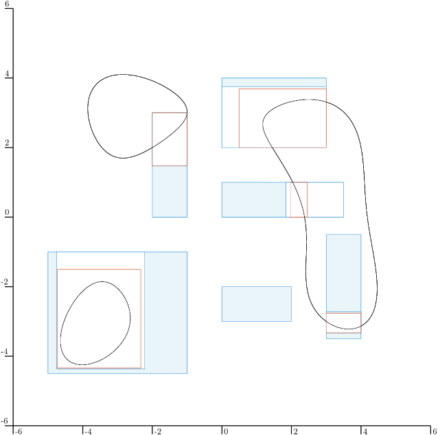
Note that the contraction may be fast but not minimal, depending on your analytic expression. Therefore, you can also combine a CtcInverse with a CtcFixpoint to apply the contraction procedure repeatedly until a fixpoint is reached on the same box. The following code corresponds to a contraction revealed in the next figure, which shows contraction cases in blue and their fixpoint counterparts in red.
z = IntervalVector([[0,3.5],[0,1]])
DefaultFigure.draw_box(z, [Color.blue(),Color.blue(.1)]) # prior to contraction
z = c.contract(z)
DefaultFigure.draw_box(z, [Color.blue(),Color.white()]) # after one CtcInverse contraction
# z == [ [1.84, 3.5] ; [0, 1] ]

# Combining CtcInverse with a CtcFixpoint:
cfix = CtcFixpoint(c)
z = c.contract(z)
DefaultFigure.draw_box(z, Color.red()) # after a fixed point contraction
# z == [ [1.84, 2.483] ; [0, 1] ]
IntervalVector z({{0,3.5},{0,1}});
DefaultFigure::draw_box(z, {Color::blue(),Color::blue(.1)}); // prior to contraction
c.contract(z);
DefaultFigure::draw_box(z, {Color::blue(),Color::white()}); // after one CtcInverse contraction
// z == [ [1.84, 3.5] ; [0, 1] ]

// Combining CtcInverse with a CtcFixpoint:
CtcFixpoint cfix(c);
c.contract(z);
DefaultFigure::draw_box(z, Color::red()); // after a fixed point contraction
// z == [ [1.84, 2.483] ; [0, 1] ]
z = IntervalVector({{0.0,3.5},{0.0,1.0}});
DefaultFigure().draw_box(z, StyleProperties({Color().blue(),Color().blue(.1)})); % prior to contraction
z = c.contract(z);
DefaultFigure().draw_box(z, StyleProperties({Color().blue(),Color().white()})); % after one CtcInverse contraction
% z == [ [1.84, 3.5] ; [0, 1] ]

% Combining CtcInverse with a CtcFixpoint:
cfix = CtcFixpoint(c);
z = c.contract(z);
DefaultFigure().draw_box(z, Color().red()); % after a fixed point contraction
% z == [ [1.84, 2.483] ; [0, 1] ]
As any other contractor, a CtcInverse can also be involved in a paver in order to reveal the constraint set:
DefaultFigure.pave([[-6,6],[-6,6]], c, 1e-2)
DefaultFigure::pave({{-6,6},{-6,6}}, c, 1e-2);
DefaultFigure().pave(IntervalVector({{-6,6},{-6,6}}), c, 1e-2);
Which produces the following output:
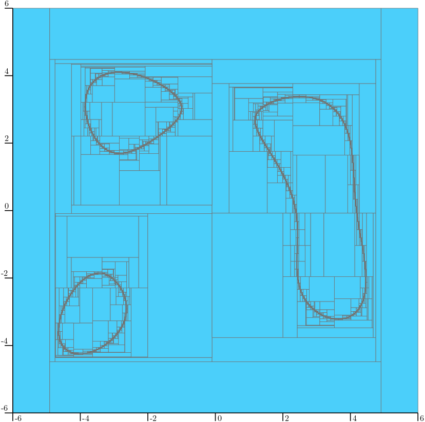
Outer approximation of the solution set for \(f(\mathbf{x})\in[50,50]\). This paving result reveals three connected subsets approximated with outer boxes. Blue parts are guaranteed not to contain solutions.
We recall that for thick solution sets, one should prefer the use of the SepInverse separator in order to get both outer and inner approximations. For instance, the solution set associated with \(f(\mathbf{x})\leqslant 50\) corresponds to:
s = SepInverse(f, [0,50])
DefaultFigure.pave([[-6,6],[-6,6]], s, 1e-2)
SepInverse s(f, {0,50});
DefaultFigure::pave({{-6,6},{-6,6}}, s, 1e-2);
s = SepInverse(f, Interval(0,50));
DefaultFigure().pave(IntervalVector({{-6,6},{-6,6}}), s, 1e-2);
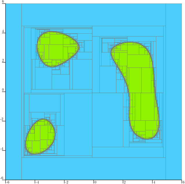
Inner and outer approximations of the solution set for \(f(\mathbf{x})\leqslant 50\), equivalent to \(f(\mathbf{x})\in[0,50]\), obtained by paving a separator SepInverse(f, [0,50]). Green parts are boxes containing only vectors consistent with the constraint.
Finally, it is easy to consider disjunction of constraints by making a union of contractors. For instance, the solution set
can be easily approximated by the following union of contractors:
cu = CtcInverse(f,50) | CtcInverse(f,150) | CtcInverse(f,250)
DefaultFigure.pave([[-6,6],[-6,6]], cu, 1e-2)
auto cu = CtcInverse(f,50) | CtcInverse(f,150) | CtcInverse(f,250);
DefaultFigure::pave({{-6,6},{-6,6}}, cu, 1e-2);
cu = CtcUnion(CtcUnion(CtcInverse(f,50), CtcInverse(f,150)), CtcInverse(f,250));
DefaultFigure().pave(IntervalVector({{-6,6},{-6,6}}), cu, 1e-2)
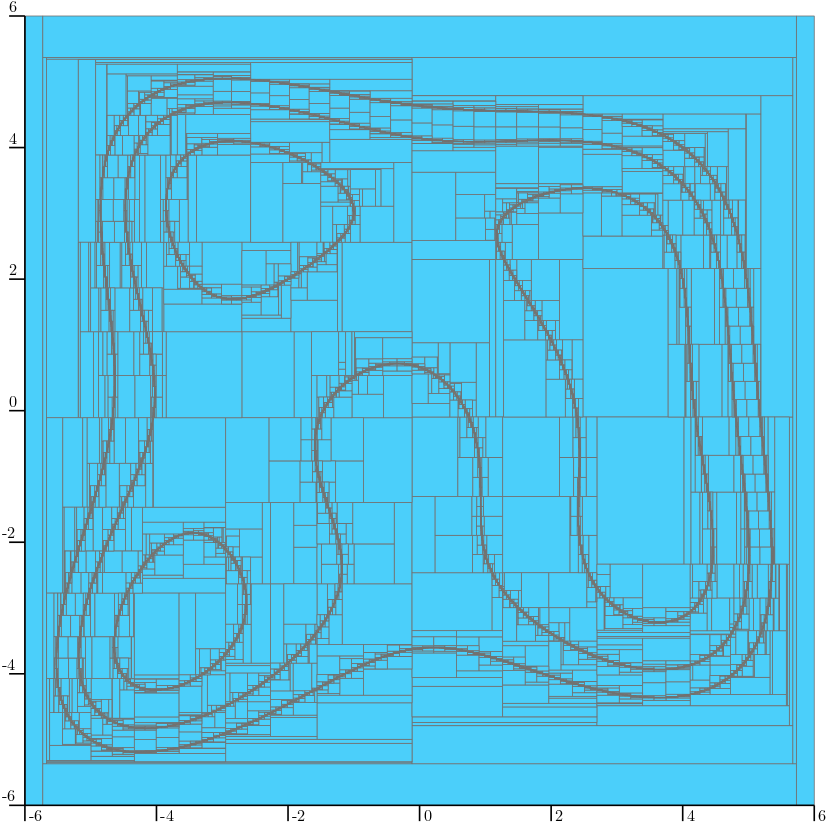
Outer approximation of the solution set \(\mathbb{X}\) for (1).
Possible usages of CtcInverse with respect to domain and codomain types
\(\mathbf{f}:\mathbb{R}^n\to \mathbb{R}^p\) is the most classical case, but Codac provides generic solutions to define a wide variety of expressions such as functions defined as \(\mathbf{f}:X\to Y\), where:
\(X\) denotes the domain of \(\mathbf{f}\) with the following cases:
\(X=\mathbb{R}\): one scalar input ;
\(X=\mathbb{R}^n\): one \(n\)-d vector input ;
\(X=\mathbb{R}^{n\times m}\): one \(n\times m\) matrix input ;
\(X=\mathbb{R}\times\mathbb{R}^{n}\times\mathbb{R}\): several types of mixed inputs, with no restrictions on order or number.
\(Y\) denotes the codomain of \(\mathbf{f}\), that can be either \(\mathbb{R}\), \(\mathbb{R}^p\) or \(\mathbb{R}^{p\times q}\).
The following table lists the combinations implemented in Codac.
The ✓ cases correspond to efficient contractions involving centered form expressions, while ✓ refer to classical forward/backward propagations.
Note that since Codac’s design is based on C++ template programming, the most generic use-cases of the CtcInverse are not available in Python or Matlab.
Output \(Y\) |
||||
\(\mathbb{R}\) - |
\(\mathbb{R}^n\) - |
\(\mathbb{R}^{r\times c}\) - |
||
Input(s) \(X\) |
\(\mathbb{R}\) |
✓ |
✓ |
✗ (C++ only) |
\(\mathbb{R}^n\) |
✓ |
✓ |
✗ (C++ only) |
|
\(\mathbb{R}^{r\times c}\) |
✓ |
✓ |
✗ (C++ only) |
|
any mixed types |
✓ |
✓ |
✗ (C++ only) |
|
NB: any mixed types does not include matrix types yet.
Output \(Y\) |
||||
\(\mathbb{R}\) - |
\(\mathbb{R}^n\) - |
\(\mathbb{R}^{r\times c}\) - |
||
Input(s) \(X\) |
\(\mathbb{R}\) |
✓ |
✓ |
✓ |
\(\mathbb{R}^n\) |
✓ |
✓ |
✓ |
|
\(\mathbb{R}^{r\times c}\) |
✓ |
✓ |
✓ |
|
any mixed types |
✓ |
✓ |
✓ |
|
Output \(Y\) |
||||
\(\mathbb{R}\) - |
\(\mathbb{R}^n\) - |
\(\mathbb{R}^{r\times c}\) - |
||
Input(s) \(X\) |
\(\mathbb{R}\) |
✓ |
✓ |
✗ (C++ only) |
\(\mathbb{R}^n\) |
✓ |
✓ |
✗ (C++ only) |
|
\(\mathbb{R}^{r\times c}\) |
✓ |
✓ |
✗ (C++ only) |
|
any mixed types |
✓ |
✓ |
✗ (C++ only) |
|
NB: any mixed types does not include matrix types yet.
Not-in constraints: CtcInverseNotIn
When the constraint is a complement constraint \(\mathbf{f}(\mathbf{x})\notin\mathbb{Y}\), Codac provides CtcInverseNotIn which internally builds a union of inverse contractors over the complementary parts of \(\mathbb{Y}\).
x = VectorVar(2)
f = AnalyticFunction([x], x[0])

# Enforce the first component not in [0,1]
c = CtcInverseNotIn(f, [0,1])

y = IntervalVector([[0.5,3],[-1,1]])
y = c.contract(y) # [[1,3],[-1,1]]
# Only the first component is constrained by the not-in condition
VectorVar x(2);
AnalyticFunction f({x}, x[0]);

// Enforce the first component not in [0,1]
CtcInverseNotIn c(f, {0,1});

IntervalVector y({{0.5,3},{-1,1}});
c.contract(y); // {{1,3},{-1,1}}
// Only the first component is constrained by the not-in condition
x = VectorVar(2);
f = AnalyticFunction({x}, x(1));

% Enforce the first component not in [0,1]
c = CtcInverseNotIn(f, Interval(0,1));

y = IntervalVector({{0.5,3},{-1,1}});
y = c.contract(y); % [[1,3],[-1,1]]
% Only the first component is constrained by the not-in condition
Miscellaneous
Access to the underlying function
The underlying analytic function can be accessed through .fnc() (useful for dimension checks or meta-programming).
x = VectorVar(2)
f = AnalyticFunction([x], x[0]-x[1])
c = CtcInverse(f, 0)
assert c.fnc().input_size() == 2
assert c.fnc().output_size() == 1
VectorVar x(2);
AnalyticFunction f({x}, x[0]-x[1]);
CtcInverse c(f, 0);
// c.fnc().input_size() == 2
// c.fnc().output_size() == 1
x = VectorVar(2);
f = AnalyticFunction({x}, x(1)-x(2));
c = CtcInverse(f, 0);
assert(c.fnc().input_size() == 2);
assert(c.fnc().output_size() == 1);
Centered form option
For some signatures (see ✓ in the table), CtcInverse can leverage centered-form
expressions to improve contraction.
The constructor exposes:
with_centered_form(default:true): enable/disable centered-form based steps.
Disabling it can be useful to reduce computation cost when forward/backward propagation is sufficient for your application, or for comparisons with the centered form.
Technical documentation
See the C++ API documentation:
CtcInverse: codac2_CtcInverse.hCtcInverseNotIn: codac2_CtcInverseNotIn.h