CAPD (rigorous numerics in dynamical systems)
Main author: Maël Godard
This page describes how to use the CAPD library with Codac. CAPD is a C++ library for rigorous numerics in dynamical systems.
To use CAPD with Codac, you first need to install the CAPD library. You can find the installation instructions on the CAPD website.
Note that as CAPD is a C++ only library, the content present in this page is only available in C++.
Installing the codac-capd extension
To install the codac-capd extension, you need to install the Codac library from its sources. This can be done by using CMake with the option WITH_CAPD=ON. For example:
cmake -DCMAKE_INSTALL_PREFIX=$HOME/ibex-lib/build_install -DCMAKE_BUILD_TYPE=Release -DWITH_CAPD=ON ..
We highly recommend to test the installation of the library with the provided tests. To do so, you can use the following command:
make test
Content
The codac-capd extension provides functions to convert CAPD objects to Codac objects and vice versa.
The functions are to_capd and to_codac. They can be used to convert the following objects:
capd::Interval\(\leftrightarrow\)codac2::Intervalcapd::IVector\(\leftrightarrow\)codac2::IntervalVectorcapd::IMatrix\(\leftrightarrow\)codac2::IntervalMatrixcapd::ITimeMap::SolutionCurve\(\rightarrow\)codac2::SlicedTube<codac2::IntervalVector>
How to use
The header of the codac-capd extension is not included by default. You need to include it manually in your code, together with the CAPD library:
#include <codac-capd.h>
#include <capd/capdlib.h>
Furthermore, you need to link the extension to your project, for instance by updating your CMakeLists.txt with:
add_executable(${PROJECT_NAME} main.cpp)
target_compile_options(${PROJECT_NAME} PUBLIC ${CODAC_CXX_FLAGS})
target_include_directories(${PROJECT_NAME} SYSTEM PUBLIC ${CODAC_INCLUDE_DIRS} ${CODAC_CAPD_INCLUDE_DIR})
target_link_libraries(${PROJECT_NAME} PRIVATE
  ${CODAC_LIBRARIES}
  ${CODAC_CAPD_LIBRARY} # linking to the codac-capd extension
  capd::capd # linking to CAPD
  Ibex::ibex
)
You can use the functions to_capd and to_codac to convert between CAPD and Codac objects as follows:
codac2::Interval codac_interval(0,2);  // Codac interval [0, 2]
capd::Interval capd_interval = to_capd(codac_interval); // convert to CAPD interval
codac2::Interval codac_interval2 = to_codac(capd_interval); // convert back to Codac interval
Example
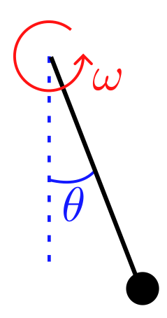
For this example we will consider the pendulum with friction.
The state variables of the pendulum are its angle \(\theta\) and its angular velocity \(\omega\). The pendulum follows the following dynamic:
where \(g\) is the gravity constant and \(l\) is the length of the pendulum.
This equation can be passed to the CAPD library as follows:
capd::IMap vectorField("par:l,g;var:t,w;fun:w,-sin(t)*g/l - 0.5*w;");

vectorField.setParameter("l",capd::Interval(2.)); // length of the pendulum equal to 2
vectorField.setParameter("g",capd::Interval(10.));  // gravity acceleration equal to 10
To solve this ODE, an IOdeSolver object is necessary.
capd::IOdeSolver solver(vectorField,20);
solver.setAbsoluteTolerance(1e-10);
solver.setRelativeTolerance(1e-10);
CAPD then uses an ITimeMap to make the link between a time step and the solution of the ODE at this time. The I here stands for Interval as the solution is an interval guaranteed to enclose the solution. Here we will integrate the ODE between \(t_0=0s\) and \(t_f=20s\).
capd::ITimeMap timeMap(solver);
capd::Interval initialTime(0.);  // initial time (t0)
capd::Interval finalTime(20.); // final time (tf)
To completly define the ODE, we need to define the initial conditions. Here we will set the initial angle to \(\theta_0=-\frac{\pi}{2}\) and the initial angular velocity to \(\omega_0=0\). For the purpose of this example, we will add a small uncertainty to the initial conditions. The initial conditions are then defined as follows:
capd::IVector c(2);
c[0] = -M_PI/2.;
c[1] = 0.;
// take some box around c
c[0] += capd::Interval(-1,1)*1e-2;
c[1] += capd::Interval(-1,1)*1e-2;

// define a doubleton representation of the interval vector c
capd::C0HORect2Set s(c);
There are then two ways to get the result of the integration depending on the use case.
If the desired result is the solution of the ODE at a given time (here say \(T=1s\)), we can do as follows:
capd::Interval T(1);
capd::IVector result = timeMap(T,s);
Be careful, this method modifies the initial set s in place.
If the desired result is the solution curve (or tube) of the ODE on the time domain \([t_0,t_f]\), we can do as follows:
capd::ITimeMap::SolutionCurve solution(initialTime);
timeMap(finalTime,s,solution);
The variable solution is the desired solution curve (or tube). The operator solution(t) gives the solution at time \(t\).
It can be converted into a Codac SlicedTube<IntervalVector> with the function to_codac. This functions takes two arguments:
the
capd::ITimeMap::SolutionCurveto convert.a
codac2::TDomainobject defining the temporal domain of the tube.
The resulting SlicedTube will have the same time domain as the one given in argument, completed with the CAPD gates. An example of conversion is :
auto tdomain = create_tdomain(Interval(0,20),0.05, true); // true to have gates
auto codac_tube = to_codac(solution, tdomain);
A full display can be done with the following code:
std::cout << "\ninitial set: " << c;
std::cout << "\ndiam(initial set): " << diam(c) << std::endl;

std::cout << "\n\nafter time=" << T << " the image is: " << result;
std::cout << "\ndiam(image): " << diam(result) << std::endl << std::endl;

DefaultFigure::set_axes(axis(0,{-2,1.5}),axis(1,{-2,3}));

DefaultFigure::draw_tube(codac_tube, ColorMap::blue_tube());
DefaultFigure::draw_tube(codac_tube, Color::black());

for (float t=0.;t<20.;t+=0.05)
  DefaultFigure::draw_box(to_codac(solution(t)), {Color::none(), Color::orange(0.5)});

DefaultFigure::draw_box(to_codac(c),Color::green());
DefaultFigure::draw_box(to_codac(result),Color::red());
The result is the following figure, with in green the initial set (\(t=0s\)) and in red the final set (\(t=20s\)). The SlicedTube is displayed in blue with a black edge for better visibility. The orange rectangles correspond to the gates (degenerate slices).
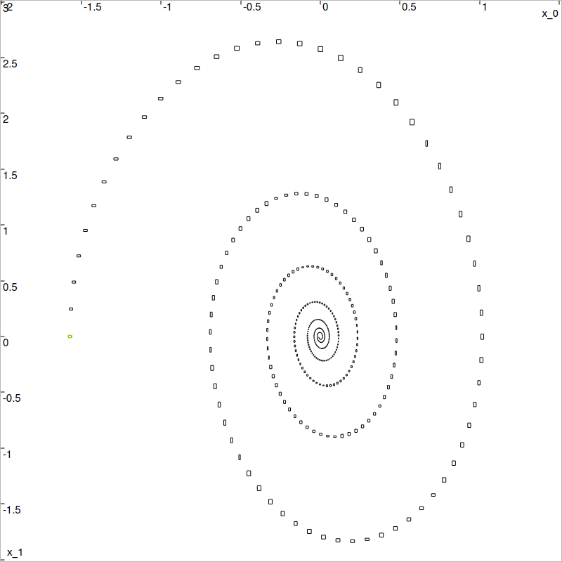
Result of the CAPD integration of the pendulum, enclosed in a Codac tube.