Lesson B: Data association

This lesson will extend the previous exercise by dealing with a data association problem together with localization: the landmarks perceived by the robot are now indistinguishable: they all look alike. The goal of this exercise is to develop our own contractor in order to solve the problem.

Introduction: indistinguishable landmarks

As before, our goal is to deal with the localization of a mobile robot for which a map of the environment is available.

It is assumed that:

• the map is static and made of point landmarks;

• the landmarks are indistinguishable (which was not the case before);

• the position of each landmark is known;

• the position of the robot is not known.

This problem often occurs when using sonars for localization, where it is difficult to distinguish a landmark from another. The challenge in this type of scenario is the difficulty of data associations, i.e. establishing feature correspondences between perceptions of landmarks and the map of these landmarks, known beforehand. This is especially the case of challenging underwater missions, for which one can reasonably assume that the detected landmarks cannot be distinguished from the other in sonar images. For instance, two different rocks may have the same aspect and dimension in the acquired images, as illustrated by the following figure.

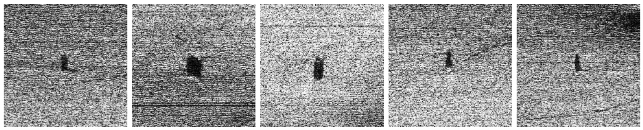
Different underwater rocks perceived with one side-scan sonar. These observations are view-point dependent and the sonar images are noisy, which makes it difficult to distinguish one rock from another only from image processing. These sonar images have been collected by the Daurade robot (DGA-TN Brest, Shom, France) equipped with a Klein 5000 lateral sonar.

Due to these difficulties, we consider that we cannot compute reliable data associations that stand on image processing of the observations. We will rather consider the data association problem together with state estimation.

Data association: formalism

Up to now, we assumed that one perceived landmark was identified without ambiguity. However, when several landmarks \(\mathbf{m}_{1}\), \(\dots\), \(\mathbf{m}_{\ell}\) exist, the observation data may not be associated: we do not know to which landmark the measurement \(\mathbf{y}\) refers. We now consider several measurements denoted by \(\mathbf{y}^i\). Hence the observation constraint has the form:

\[\begin{split}\left\{ \begin{array}{l} \mathbf{g}\big(\mathbf{x},\mathbf{y}^{i},\mathbf{m}^{i}\big)=\mathbf{0},\\ \big(\mathbf{m}^{i}\in[\mathbf{m}_{1}]\big)\vee\dots\vee\big(\mathbf{m}^{i}\in[\mathbf{m}_{\ell}]\big), \end{array}\right.\end{split}\]

with \(\mathbf{m}^{i}\) the unidentified landmark of the observation \(\mathbf{y}^i\). The \(\vee\) notation expresses the logical disjunction or. Equivalently, the system can be expressed as:

\[\begin{split}\left\{ \begin{array}{l} \mathbf{g}\big(\mathbf{x},\mathbf{y}^{i},\mathbf{m}^{i}\big)=\mathbf{0},\\ \mathbf{m}^{i}\in\mathbb{M}=\left\{ [\mathbf{m}_{1}],\dots,[\mathbf{m}_{\ell}]\right\}, \end{array}\right.\end{split}\]

where \(\mathbb{M}\) is the bounded map of the environment: the set of all landmarks represented by their bounded positions. In other words, we do not know the right parameter vector \(\mathbf{m}_{1}\), \(\dots\), \(\mathbf{m}_{\ell}\) associated with the observation \(\mathbf{y}^i\). This is a problem of data association. The following figure illustrates \(\mathbb{M}\) with the difficulty to differentiate landmarks in underwater extents.

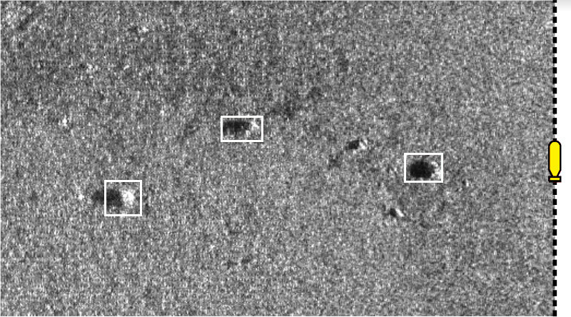
The yellow robot, equipped with a side-scan sonar, perceives at port side some rocks \(\mathbf{m}^{i}\) lying on the seabed. The rocks, that can be used as landmarks, are assumed to belong to small georeferenced boxes \(\mathbb{M}\) enclosing uncertainties on their positions. The robot is currently not able to make any difference between the rocks, as it is typically the case in underwater extents when acoustic sensors are used to detect features.

In this exercise, the data association problem is solved together with state estimation, without image processing. The constraint \(\mathbf{g}\big(\mathbf{x},\mathbf{y}^{i},\mathbf{m}^{i}\big)=\mathbf{0}\) has been solved in Lesson A: Static range-and-bearing localization, it remains to deal with the constraint \(\mathbf{m}^{i}\in\mathbb{M}\). We will call it the constellation constraint.

The constellation constraint and its contractor

When solving a problem with a constraint propagation approach, we may not have the contractors at hand for dealing with all the involved constraints. In this lesson for instance, we assume that we do not have a contractor for dealing with this constellation constraint. The goal of the following exercise is to see how to build our own contractor. We will see that it is easy to extend our framework with new contractors, without loss of generality.

We now focus on the constellation constraint without relation with the other equations. The constraint is expressed by \(\mathcal{L}_{\mathbb{M}}\left(\mathbf{a}\right)~:~\mathbf{a}\in\mathbb{M}\).

Let us consider a constellation of \(\ell\) landmarks of \(\mathbb{IR}^{2}\), \(\mathbb{M}=\{[\mathbf{m}_{1}],\dots,[\mathbf{m}_{\ell}]\}\), and a box \([\mathbf{a}]\in\mathbb{IR}^2\). Our goal is to compute the smallest box containing \(\mathbb{M}\cap[\mathbf{a}]\). In other words, we want to contract the box \([\mathbf{a}]\) so that we only keep the best envelope of the landmarks that are already included in \([\mathbf{a}]\). An illustration is provided by the following figures:

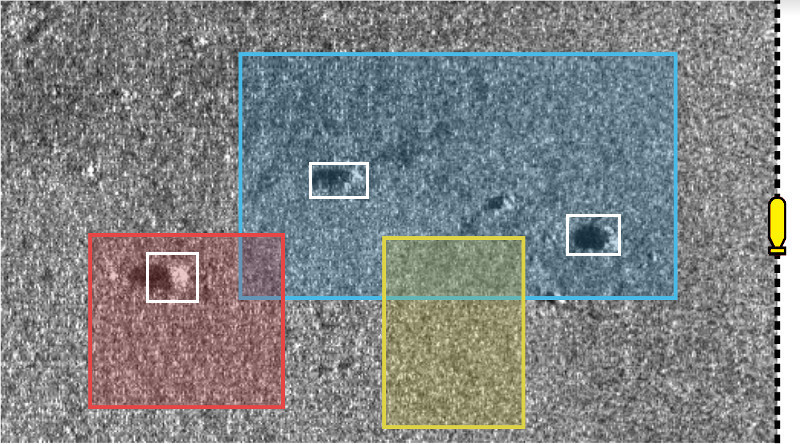
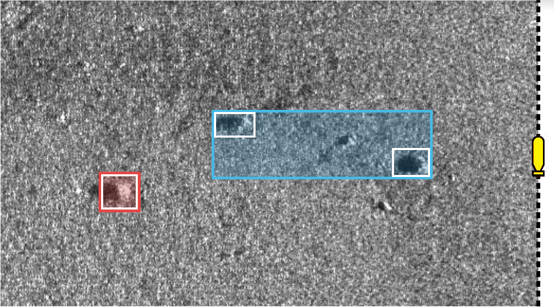
Illustration of the constellation contractor, before and after the contraction step. The set \(\mathbb{M}\) of landmarks is depicted by white boxes. Colored boxes depict several cases of \([\mathbf{a}]\), before and after contraction. In this example, the red perception leads to a reliable identification since the box contains only one item of \(\mathbb{M}\). We recall that the sonar image in background is not involved in this contraction: it is only used for understanding the application of this contractor. Here, the operator is reliable as it does not remove any significant rock.

The definition of the contractor is given by:

\[\mathcal{C}_\mathbb{M}\left(\left[\mathbf{a}\right]\right)=\bigsqcup_{j=1}^{\ell}\big(\left[\mathbf{a}\right]\cap[\mathbf{m}_{j}]\big),\]

where \(\bigsqcup\), called squared union, returns the smallest box enclosing the union of its arguments.

Exercise

(you may insert your code in the previous Lesson A)

B.1. We can now build our own contractor class, MyCtc. To do it, we have to derive the base class Ctc_IntervalVector (in Python/Matlab) or Ctc<MyCtc,IntervalVector> (in C++) that is common to all contractors on boxes. You can start from the following new class:

PythonC++

class MyCtc(Ctc_IntervalVector):

  def __init__(self, M_: list):
    Ctc_IntervalVector.__init__(self, 2) # the contractor acts on 2d boxes
    self.M = M_                          # attribute needed later on for the contraction

  def contract(self, a):

    # Insert contraction formula here (question B.2)

    return a # in Python, the updated value must be returned

Note that:

• M represents the set \(\mathbb{M}\), made of 2d IntervalVector objects;

• a (in .contract()) is the box \([\mathbf{a}]\) (2d IntervalVector) to be contracted.

B.2. Propose a simple implementation of the method .contract() for contracting \([\mathbf{a}]\) as:

\[\mathcal{C}_\mathbb{M}\left(\left[\mathbf{a}\right]\right)=\bigsqcup_{j=1}^{\ell}\big(\left[\mathbf{a}\right]\cap[\mathbf{m}_{j}]\big)\]

The user manual may help you to compute operations on sets such as unions or intersections, appearing in the formula. Note that you cannot change the definition of the .contract() method.

PythonC++

  def contract(self, a):
    u = IntervalVector.empty(2)
    for mi in self.M:
      u |= a & mi
    a = IntervalVector(u)
    return a

B.3. Test your contractor with:

• a set \(\mathbb{M}=\big\{(1.5,2.5)^\intercal,(3,1)^\intercal,(2,2)^\intercal,(2.5,3)^\intercal,(3.5,2)^\intercal,(4,1)^\intercal,(1.5,0.5)^\intercal\big\}\), all boxes inflated by \([-0.05,0.05]\);

• three boxes to be contracted: \([\mathbf{a}^1]=([1.25,3],[1.6,2.75])^\intercal\), \([\mathbf{a}^2]=([2,3.5],[0.6,1.2])^\intercal\), and \([\mathbf{a}^3]=([1.1,3.25],[0.2,1.4])^\intercal\).

You can try your contractor with the following code:

PythonC++

# M = [ ...
for Mi in M:
  Mi.inflate(0.05)

# a1 = IntervalVector([ ...
# a2 = IntervalVector([ ...
# a3 = IntervalVector([ ...

ctc_constell = MyCtc(M)

a1 = ctc_constell.contract(a1)
a2 = ctc_constell.contract(a2)
a3 = ctc_constell.contract(a3)

PythonC++

M = [
  IntervalVector([1.5,2.5]),
  IntervalVector([3,1]),
  IntervalVector([2,2]),
  IntervalVector([2.5,3]),
  IntervalVector([3.5,2]),
  IntervalVector([4,1]),
  IntervalVector([1.5,0.5])
]

for Mi in M:
  Mi.inflate(0.05)

a1 = IntervalVector([[1.25,3],[1.6,2.75]])
a2 = IntervalVector([[2,3.5],[0.6,1.2]])
a3 = IntervalVector([[1.1,3.25],[0.2,1.4]])

ctc_constell = MyCtc(M)

a1 = ctc_constell.contract(a1)
a2 = ctc_constell.contract(a2)
a3 = ctc_constell.contract(a3)

print(a1, '\n', a2, '\n', a3)

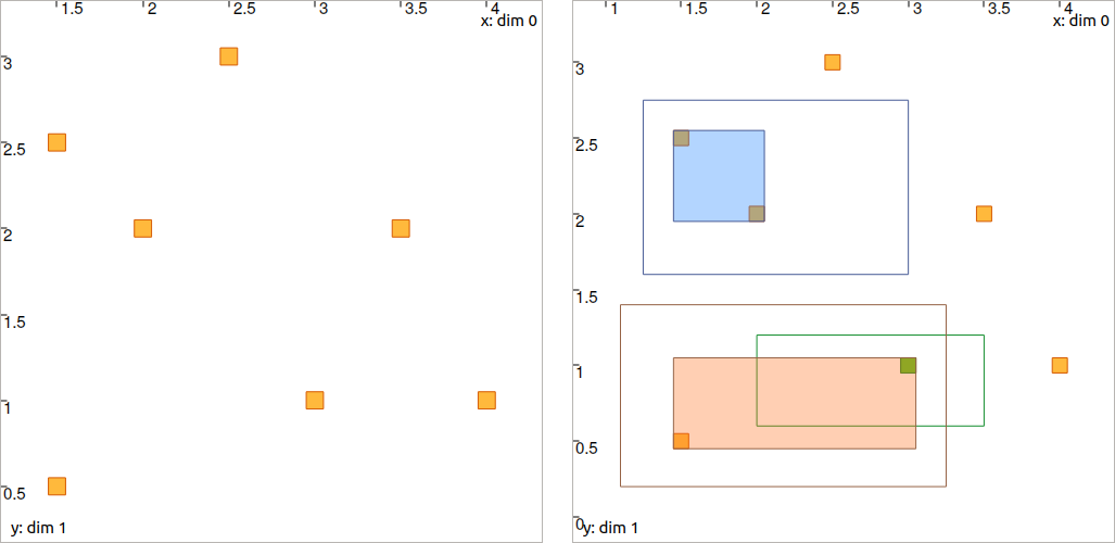
Expected result for Question B.3 (you may verify your results only by printing boxes values). Non-filled boxes are initial domains before contraction. Filled boxes are contracted domains. The green one, \([\mathbf{a}^3]\), is identified since it contains only one item of the constellation \(\mathbb{M}\): there is no ambiguity about the constellation point represented by the box \([\mathbf{a}^3]\).

Numerical results are given:

[a1]: ([1.45, 2.05] ; [1.95, 2.55])    (blue box)
[a2]: ([2.95, 3.05] ; [0.95, 1.05])    (green box)
[a3]: ([1.45, 3.05] ; [0.45, 1.05])    (red box)

Application for localization

This contractor is really simple, but it will help us to solve more complex problems.

We now have all the material to solve the full problem of state estimation with data association.

We will localize the robot in the map \(\mathbb{M}\) created in Question B.3.

Exercise

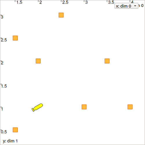
B.4. In your code, define a robot with the following pose \(\mathbf{x}=\left(2,1,\pi/6\right)^\intercal\) (the same as in Lesson A).

PythonC++

x_truth = Vector([2,1,PI/6])

B.5. Display the robot and the landmarks in a graphical view with:

PythonC++

DefaultFigure.set_axes(axis(0,[1,4.5]), axis(1,[0,3.5]))
DefaultFigure.draw_tank(x_truth, 0.4, [Color.black(),Color.yellow()])
for mi in M:
  DefaultFigure.draw_box(mi, [Color.dark_green(),Color.green()])

You should obtain this result.

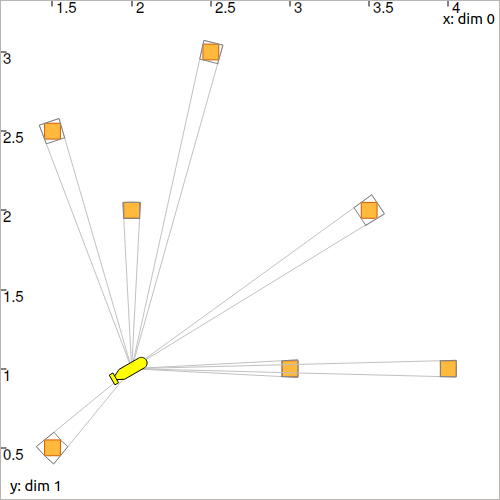
B.6. We will generate a set of range-and-bearing measurements made by the robot. For this, we will use an observation function to compute the range and bearing between a state x and a landmark mi:

PythonC++

def g(x, mi):
  r = sqrt(sqr(mi[0]-x[0]) + sqr(mi[1]-x[1]))
  b = atan2(mi[1]-x[1], mi[0]-x[0]) - x[2]
  return IntervalVector([r,b]).inflate([0.02,0.02])

The returned value is a vector of [range]×[bearing] interval values.

Compute and display the measurements in the view with .draw_pie(), as we did in the previous lesson. The identity (i.e. the position) of each landmark will be given in the last components of the observation vectors:

PythonC++

obs = []
for mi in M:
  obs.append(cart_prod(g(x_truth,mi),mi))
  # We append the position of the landmark to the measurement
  # yi = [range]×[bearing]×[2d position]

for yi in obs:
  DefaultFigure.draw_pie(x_truth.subvector(0,1), yi[0],     x_truth[2]+yi[1], Color.red())
  DefaultFigure.draw_pie(x_truth.subvector(0,1), yi[0] | 0, x_truth[2]+yi[1], Color.light_gray())

You should obtain a figure similar to this one:

State estimation without data association

We will go step by step and not consider the data association problem for the moment.

We will first reuse the fixpoint method of the previous Lesson, and apply it on this set of observations.

Exercise

D.7. Use a second fixpoint method to perform the state estimation of the robot (the contraction of \([\mathbf{x}]\)) by considering iteratively all the observations.

We will assume that:

• the identity (the position) of the related landmarks is known;

• the heading \(x_3\) of the robot is known.

In the code, the identity of each landmark is known in the sense that a measurement v_obs[i] refers to a landmark M[i].

PythonC++

def ctc_one_obs(x,yi,mi,ai,di):
  mi,x,di = ctc_minus.contract(mi,x,di)
  x[2],yi[1],ai = ctc_plus.contract(x[2],yi[1],ai)
  di[0],di[1],yi[0],ai = ctc_polar.contract(di[0],di[1],yi[0],ai)
  return x,yi,mi,ai,di

def ctc_all_obs(x):
  for yi in obs:
    # Intermediate variables for each observation;
    ai = Interval()
    di = IntervalVector(2)
    mi = yi.subvector(2,3) # the identity (position) of the landmark is known
    # Running a fixpoint for each observation
    x,yi,mi,ai,di = fixpoint(ctc_one_obs, x,yi,mi,ai,di)
  return x

x = cart_prod([-oo,oo],[-oo,oo],x_truth[2])
x = fixpoint(ctc_all_obs, x)

B.8. Display the resulted contracted box \([\mathbf{x}]\) with:

PythonC++

print(x)
DefaultFigure.draw_box(x) # does not display anything if unbounded

You should obtain this result in black (considering uncertainties proposed in Question B.6):

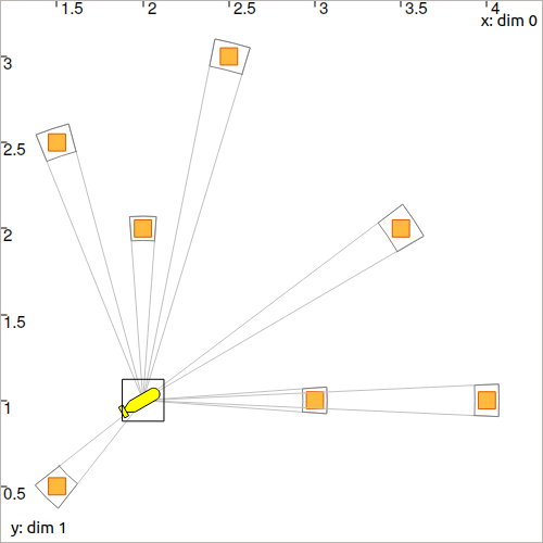
Range-and-bearing static localization, with several observations of identified landmarks.

State estimation with data association

We now assume that the identities of the landmarks are not known. This means that we will not use the third and fourth components of the observation vectors yi anymore in the resolution of the problem.

Exercise

B.9. Update the fixpoint functions for solving the state estimation together with the data association problem. The algorithm should now involve the mi objects as well as the new contractor constellation contractor that you developed in Questions B1–3.

You should obtain exactly the same result as in Question B.8.

PythonC++

ctc_constell = MyCtc(M)
x = cart_prod([-oo,oo],[-oo,oo],x_truth[2]) # reset for testing

def ctc_one_obs_datasso(x,yi,mi,ai,di):
  mi,x,di = ctc_minus.contract(mi,x,di)
  x[2],yi[1],ai = ctc_plus.contract(x[2],yi[1],ai)
  di[0],di[1],yi[0],ai = ctc_polar.contract(di[0],di[1],yi[0],ai)
  # ==== Added contractor ====
  mi = ctc_constell.contract(mi) # new contractor for data association
  # ==========================
  return x,yi,mi,ai,di

def ctc_all_obs_datasso(x):
  for yi in obs:
    ai = Interval()
    di = IntervalVector(2)
    # ==== Changed domain ====
    mi = IntervalVector(2) # the identity (position) of the landmark is not known
    # ========================
    x,yi,mi,ai,di = fixpoint(ctc_one_obs_datasso, x,yi,mi,ai,di)
  return x

x = fixpoint(ctc_all_obs_datasso, x)

B.11. Same result means that the data association worked: each measurement has been automatically associated to the correct landmark without ambiguity.

We can now look at the set m containing the associations. If one \([\mathbf{m}^i]\) contains only one item of \(\mathbb{M}\), then it means that the landmark of the measurement \(\mathbf{y}^i\) has been identified.

We will draw a point in the middle of each \([\mathbf{m}^i]\) that contains only one item of \(\mathbb{M}\).

In Question B.3, we defined \(\mathbb{M}\) as a set of boxes with a width of \(2\times 0.05\). Then, if one box \([\mathbf{m}^i]\) has a maximal diameter that is less than \(0.1\), it means that it contains one single item of \(\mathbb{M}\).

This can be verified in the main contraction loop:

PythonC++

    if mi.max_diam() <= 1:
      DefaultFigure.draw_point(mi.mid())

Expected result:

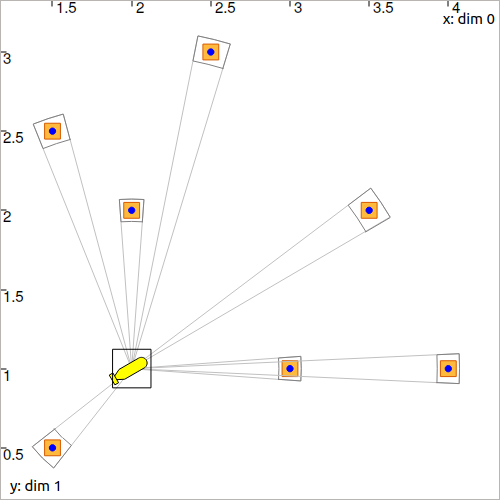
All the boxes have been identified.

Conclusion

This association has been done only by merging all information together. We define contractors from the equations of the problem, and let the information propagate in the domains. This has led to a state estimation solved concurrently with a data association.

In the next lessons, we will go a step further by making the robot move. This will introduce differential constraints, and a new domain for handling uncertain trajectories: tubes.

Related content

Related publication

Set-membership state estimation by solving data association

S. Rohou, B. Desrochers, L. Jaulin

ICRA: IEEE International Conference on Robotics and Automation, 2020.

Download the paper