The Ellipsoid class

Main author: Morgan Louédec

This page describes the Ellipsoid classes used in Codac 2 as well as some functions with ellipsoids. Additional mathematical information is provided here.

Class Ellipsoid

The Ellipsoid class can be used to declare a n-dimensional ellipsoid. The ellipsoid is defined by a center point \(\boldsymbol{\mu}\) and a shape matrix \(\boldsymbol{\varGamma}\). Ellipsoids can be drawn in VIBES via the .draw_ellipsoid function, as illustrated by Figure 1.

PythonC++

# Init drawing figure
fig1 = Figure2D('Linear and nonlinear mappings', GraphicOutput.VIBES)
fig1.set_axes(axis(0, [-0.1, 1.3]), axis(1, [-1.2, 0.2]))
fig1.set_window_properties([0, 100], [500, 500])

mu = Vector([1., 0.])
G = Matrix([[0.05, 0.0],
          [0.,   0.05]])
e1 = Ellipsoid(mu, G)

fig1.draw_ellipsoid(e1, [Color.red(), Color.red(0.3)]) # drawing

Linear and nonlinear mappings

Linear and nonlinear mappings can be applied on ellipsoids. For every ellipsoid \(ex\), square matrix \(A\) and vector \(b\), the function unreliable_linear_mapping compute the ellipsoid \(ey=A\cdot ex + b\).

Nonlinear mappings can be declared with the AnalyticFunction class. For every ellipsoid \(ex\) and nonlinear mapping \(h\), the function nonlinear_mapping compute an ellipsoid \(ey\) that enclose the image of \(ex\) by \(h\) such that \(h(ex)\in ey\)

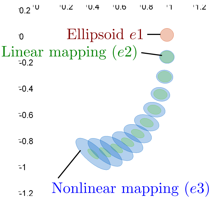
Figure 1 - Illustration of successive linear and nonlinear mappings on ellipsoids

PythonC++

# declare nonlinear mappings
x = VectorVar(2)
h = AnalyticFunction ([x], vec(x[0] + 0.1 * x[1], -0.2 * sin(x[0]) + 0.9 * x[1]))

# linear mapping
N = 10
e2 = Ellipsoid(e1)
for i in range(0,N):
    A = h.diff(e2.mu).mid()
    b = Vector(h.eval(e2.mu).mid() - A * e2.mu)
    e2 = unreliable_linear_mapping(e2, A, b)
    fig1.draw_ellipsoid(e2, [Color.green(), Color.green(0.3)])

# nonlinear mapping
e3 = Ellipsoid(e1)
for i in range(0,N):
    e3 = nonlinear_mapping(e3, h)
    fig1.draw_ellipsoid(e3, [Color.blue(), Color.blue(0.3)])

Projection of the ellipsoids

One can illustrate high dimensional ellipsoids with 2D projection. In Codac, the projection is made by the Figure2D object via the .draw_ellipsoid function : the ellipsoid is projected on the plane (0,i,j), where the axis i and j are specified via the .set_axes function of the figure.

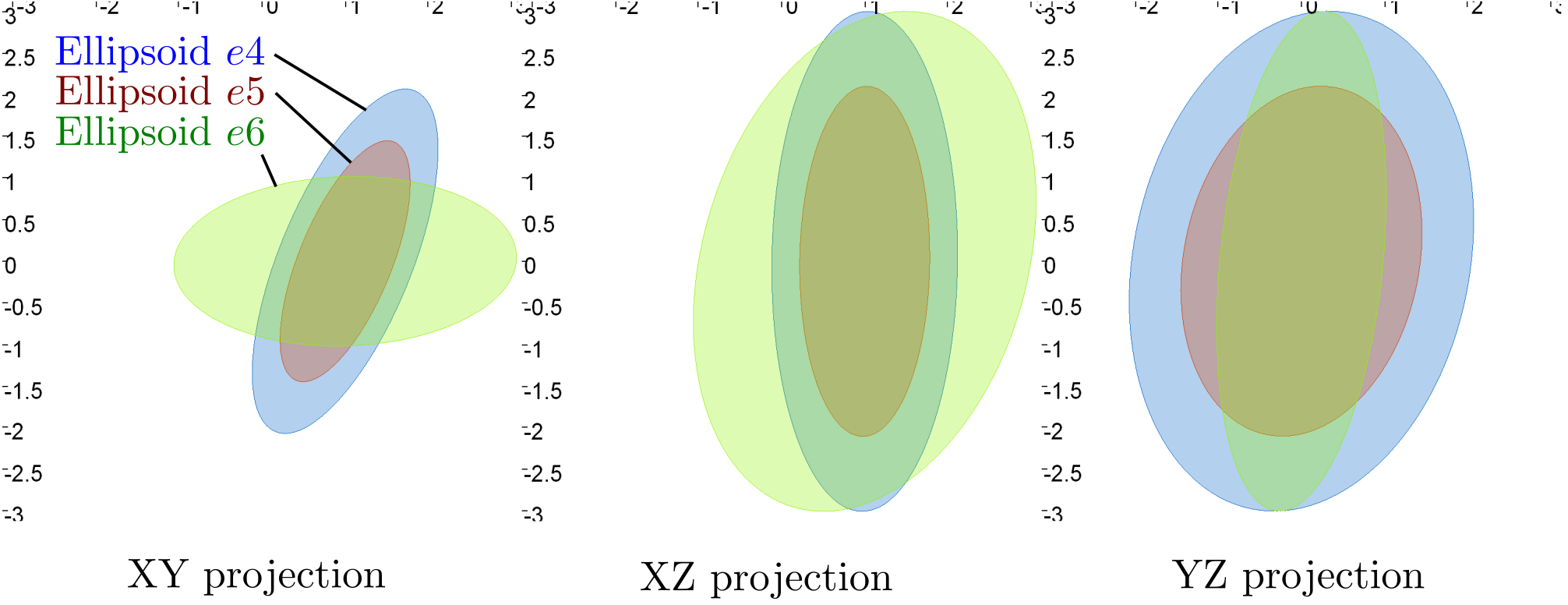
Figure 2 - Projections of the ellipsoids \(e4\), \(e5\) and \(e6\) in the 3D XYZ space

PythonC++

mu4 = Vector([1., 0., 0.])
G4 = Matrix([[1.,  0.5, 0.],
           [0.5, 2.,  0.2],
           [0.,  0.2, 3.]])
e4 = Ellipsoid(mu4, G4)

G5 = 0.7 * G4
e5 = Ellipsoid(mu4, G5)

G6 = Matrix([[2., 0.,  0.5],
           [0., 1.,  0.2],
           [0., 0.2, 3.]])
e6 = Ellipsoid(mu4, G6)

fig2 = Figure2D('Projected ellipsoid xy', GraphicOutput.VIBES)
fig3 = Figure2D('Projected ellipsoid yz', GraphicOutput.VIBES)
fig4 = Figure2D('Projected ellipsoid xz', GraphicOutput.VIBES)

fig2.set_window_properties([700, 100], [500, 500])
fig3.set_window_properties([1200, 100], [500, 500])
fig4.set_window_properties([0, 600], [500, 500])

fig2.set_axes(axis(0, [-3, 3]), axis(1, [-3, 3]))
fig3.set_axes(axis(1, [-3, 3]), axis(2, [-3, 3]))
fig4.set_axes(axis(0, [-3, 3]), axis(2, [-3, 3]))

fig2.draw_ellipsoid(e4, [Color.blue(), Color.blue(0.3)])
fig3.draw_ellipsoid(e4, [Color.blue(), Color.blue(0.3)])
fig4.draw_ellipsoid(e4, [Color.blue(), Color.blue(0.3)])

fig2.draw_ellipsoid(e5, [Color.red(), Color.red(0.3)])
fig3.draw_ellipsoid(e5, [Color.red(), Color.red(0.3)])
fig4.draw_ellipsoid(e5, [Color.red(), Color.red(0.3)])

fig2.draw_ellipsoid(e6, [Color.green(), Color.green(0.3)])
fig3.draw_ellipsoid(e6, [Color.green(), Color.green(0.3)])
fig4.draw_ellipsoid(e6, [Color.green(), Color.green(0.3)])

Inclusion tests

The function .is_concentric_subset can test if two concentric ellipsoids are strictly included in each other. The function return a BoolInterval that can be: [ true ] if the inclusion is verified / [ true, false ] if the method is not able to conclude

PythonC++

print('\nInclusion test e5 in e4: ', e5.is_concentric_subset(e4))
print('\nInclusion test e4 in e5: ', e4.is_concentric_subset(e5))
print('\nInclusion test e4 in e6: ', e6.is_concentric_subset(e4))
print('\nInclusion test e5 in e6: ', e5.is_concentric_subset(e6))

Degenerated Ellipsoids & singular mappings

It is also possible to have Degenerated Ellipsoids and to apply singular mappings on ellipsoids. There functionalities are handled by the Ellipsoid class and the nonlinear_mapping function

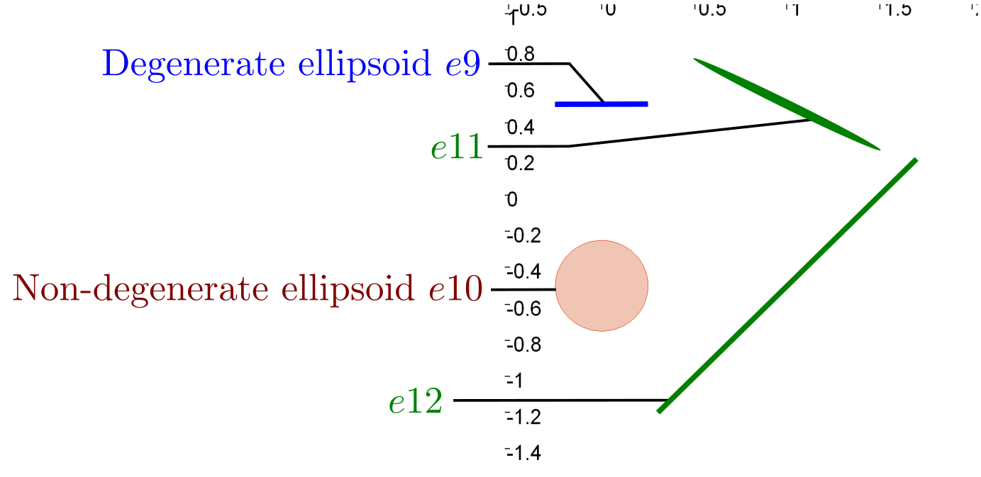
Figure 3 - Singular cases. \(e11\) is the image of \(e9\) by the nonlinear mapping \(h2\). The degenerate ellipsoid \(e12\) is the image of \(e10\) by the singular mapping \(h3\)

PythonC++

fig5 = Figure2D('singular mappings and degenerated ellipsoids', GraphicOutput.VIBES)
fig5.set_axes(axis(0, [-0.5, 2]), axis(1, [-1.5, 1.]))
fig5.set_window_properties([700, 600], [500, 500])

e9 = Ellipsoid(Vector([0., 0.5]), Matrix([[0.25, 0.],
                                        [0.,   0.]]))
e10 = Ellipsoid(Vector([0., -0.5]), Matrix([[0.25, 0.],
                                          [0.,   0.25]]))

fig5.draw_ellipsoid(e9, [Color.blue(), Color.red(0.3)])
fig5.draw_ellipsoid(e10, [Color.red(), Color.red(0.3)])

h2 = AnalyticFunction([x], vec(x[0] + 0.5 * x[1] + 0.75, -0.5 * sin(x[0]) + 0.9 * x[1] + 0.1*0.5))
h3 = AnalyticFunction([x], vec(x[0] + 0.5 * x[1] + 1.25, x[0] + 0.5 * x[1]-0.25))

e11 = nonlinear_mapping(e9, h2)
e12 = nonlinear_mapping(e10, h3)

fig5.draw_ellipsoid(e11, [Color.green(), Color.green(0.3)])
fig5.draw_ellipsoid(e12, [Color.green(), Color.green(0.3)])

print('\nDegenerate ellipsoid e9 (blue):\n', e9)
print('\nImage of degenerated ellipsoid e11 (green):\n', e11)
print('\nNon-degenerate ellipsoid e10 (red):\n', e10)
print('\nImage of singular mapping e12 (green):\n', e12)

Stability analysis

The function stability_analysis can compute a bassin of attraction for discrete time systems.

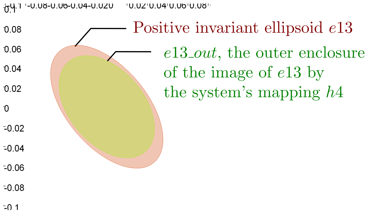
Figure 6 - Stability analysis for the discrete system \(\boldsymbol{x}_{k+1} = \boldsymbol{h4}\left(\boldsymbol{x}_k\right)\)

PythonC++

# TODO in the code