Affine transformation estimation

The affine_transformation() functions allow to compute the affine transformation (translation, rotation, scaling) that best aligns an ordered set of 2d points src with another set dst. This transformation is obtained using Singular Value Decomposition (SVD). Please note that these functions do not employ any guaranteed calculation, and the result is only an approximation that can be used for certain applications such as robotics.

The output is an Affine2d object from the Eigen library, fully available in C++. However, the Python binding of this class is only partial.

Constraints and Limitations

• Number of points: the vectors src and dst must contain the same number of points (at least 2 points are required to determine a unique transformation).

• Optimal alignment: the transformation is computed using a least-squares criterion, meaning it minimizes the mean squared error between the transformed points of src and those of dst.

• Noise sensitivity: in the presence of noise in the data, results may be affected, and pre-processing may be necessary.

• No projective transformations: this function cannot estimate projective or homographic transformations; it is limited to affine transformations.

Usage

Inputs src and dst can be provided either as a list of 2d points, or with sampled trajectories. The ordering of the points in these lists matters: every i-th point in the first list must correspond to the i-th point in the other.

PythonC++

def affine_transformation(src, dst):
# with src/dst: two lists of Vector objects, or two SampledVectorTraj objects

The following example estimates a transformation between two sampled trajectories.

PythonC++

# Building the src trajectory analytically

t = ScalarVar()
f_src = AnalyticFunction([t], [
  cos(2*t)+0.1*cos(10*t),
  2*sin(t)+0.1*sin(10*t)
])

src = AnalyticTraj(f_src,[-1,3]).sampled(0.01)

# The dst trajectory is obtained analytically with a
# transformation described by the parameters:

a = PI + PI/3 # rotation angle
b = 2.5 # scaling
T = Vector([ -3.2, 2.5 ]) # translation
f_dst = AnalyticFunction([t], [
  b*cos(a)*f_src(t)[0]-b*sin(a)*f_src(t)[1] + T[0] + 0.05*cos(100*t),
  b*sin(a)*f_src(t)[0]+b*cos(a)*f_src(t)[1] + T[1] + 0.05*sin(100*t)
])

dst = AnalyticTraj(f_dst,[-1,3]).sampled(0.01)

# Computing the transformation

tr = affine_transformation(src, dst)

# Reconstructing the dst trajectory using the estimated transformation

dst_estim = SampledVectorTraj()
for ti,src_i in src:
  dst_estim.set(ti, tr*src_i)

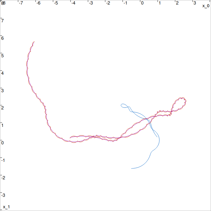
Plot of the src (blue), noised dst (red) and estimated dst_estim (purple) trajectories. dst_estim fits the initial dst trajectory.

Note that transformation values can be obtained from the Affine2d object using:

PythonC++

s = tr.linear().col(0).norm()   # scaling value
R = tr.linear() / s             # rotation matrix
angle = atan2(R(1,0), R(0,0))
T = tr.translation()            # translation vector

See Also

• Eigen::JacobiSVD for more details on the SVD decomposition used.

• Space transformations to understand affine transformation representation in Eigen.