See also
This manual refers to Codac v1, but a new v2 implementation is currently in progress… an update of this manual will be available soon. See more.
Codac: constraint-programming for robotics
Codac (Catalog Of Domains And Contractors) is a C++/Python library providing tools for constraint programming over reals, trajectories and sets. It has many applications in state estimation or robot localization.
In a nutshell, Codac is a constraint programming framework providing tools to easily solve a wide range of problems.
Keywords
|
|
|
Getting started: 2 minutes to Codac
We only have to define domains for our variables and a set of contractors to implement our constraints. The core of Codac stands on a Contractor Network representing a solver.
In a few steps, a problem is solved by
Defining the initial domains (boxes, tubes) of our variables (vectors, trajectories)
Take contractors from a catalog of already existing operators, provided in the library
Add the contractors and domains to a Contractor Network
Let the Contractor Network solve the problem
Obtain a reliable set of feasible variables
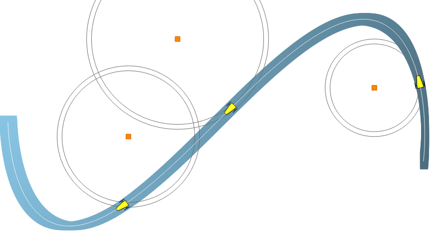
The problem is defined by classical state equations:
where \(\mathbf{u}(t)\) is the input of the system, known with some uncertainties. \(\mathbf{f}\) and \(g\) are non-linear functions.
We have three variables evolving with time: the trajectories \(\mathbf{x}(t)\), \(\mathbf{v}(t)=\dot{\mathbf{x}}(t)\), \(\mathbf{u}(t)\). We define three tubes to enclose them:
dt = 0.01                                         # timestep for tubes accuracy
tdomain = Interval(0, 3)                          # temporal limits [t_0,t_f]=[0,3]

x = TubeVector(tdomain, dt, 4)                    # 4d tube for state vectors
v = TubeVector(tdomain, dt, 4)                    # 4d tube for derivatives of the states
u = TubeVector(tdomain, dt, 2)                    # 2d tube for inputs of the system
float dt = 0.01;                                  // timestep for tubes accuracy
Interval tdomain(0, 3);                           // temporal limits [t_0,t_f]=[0,3]

TubeVector x(tdomain, dt, 4);                     // 4d tube for state vectors
TubeVector v(tdomain, dt, 4);                     // 4d tube for derivatives of the states
TubeVector u(tdomain, dt, 2);                     // 2d tube for inputs of the system
We assume that we have measurements on the headings \(\psi(t)\) and the speeds \(\vartheta(t)\), with some bounded uncertainties defined by intervals \([e_\psi]=[-0.01,0.01]\), \([e_\vartheta]=[-0.01,0.01]\):
x[2] = Tube(measured_psi, dt).inflate(0.01)       # measured_psi is a set of measurements
x[3] = Tube(measured_speed, dt).inflate(0.01)
x[2] = Tube(measured_psi, dt).inflate(0.01);      // measured_psi is a set of measurements
x[3] = Tube(measured_speed, dt).inflate(0.01);
Finally, we define the domains for the three range-only observations \((t_i,y_i)\) and the position of the landmarks. The distances \(y_i\) are bounded by the interval \([e_y]=[-0.1,0.1]\).
e_y = Interval(-0.1,0.1)
y = [Interval(1.9+e_y), Interval(3.6+e_y), \      # set of range-only observations
     Interval(2.8+e_y)]
b = [[8,3],[0,5],[-2,1]]                          # positions of the three 2d landmarks
t = [0.3, 1.5, 2.0]                               # times of measurements
Interval e_y(-0.1,0.1);
vector<Interval> y = {1.9+e_y, 3.6+e_y, 2.8+e_y}; // set of range-only observations
vector<Vector>   b = {{8,3}, {0,5}, {-2,1}};      // positions of the three 2d landmarks
vector<double>   t = {0.3, 1.5, 2.0};             // times of measurements
The distance function \(g(\mathbf{x},\mathbf{b})\) between the robot and a landmark corresponds to the CtcDist contractor provided in the library. The evolution function \(\mathbf{f}(\mathbf{x},\mathbf{u})=\big(x_4\cos(x_3),x_4\sin(x_3),u_1,u_2\big)\) can be handled by a custom-built contractor:
ctc_f = CtcFunction(
  Function("v[4]", "x[4]", "u[2]",
           "(v[0]-x[3]*cos(x[2]) ; v[1]-x[3]*sin(x[2]) ; v[2]-u[0] ; v[3]-u[1])"))
CtcFunction ctc_f(
  Function("v[4]", "x[4]", "u[2]",
           "(v[0]-x[3]*cos(x[2]) ; v[1]-x[3]*sin(x[2]) ; v[2]-u[0] ; v[3]-u[1])"));
cn = ContractorNetwork()   # creating a network

cn.add(ctc_f, [v, x, u])   # adding the f constraint

for i in range (0,len(y)): # we add the observ. constraint for each range-only measurement

  p = cn.create_interm_var(IntervalVector(4)) # intermed. variable (state at t_i)

  # Distance constraint: relation between the state at t_i and the ith beacon position
  cn.add(ctc.dist, [cn.subvector(p,0,1), b[i], y[i]])

  # Eval constraint: relation between the state at t_i and all the states over [t_0,t_f]
  cn.add(ctc.eval, [t[i], p, x, v])
ContractorNetwork cn;        // creating a network
cn.add(ctc_f, {v, x, u});    // adding the f constraint

for(int i = 0 ; i < 3 ; i++) // we add the observ. constraint for each range-only measurement
{
  IntervalVector& p = cn.create_interm_var(IntervalVector(4)); // intermed. variable (state at t_i)

  // Distance constraint: relation between the state at t_i and the ith beacon position
  cn.add(ctc::dist, {cn.subvector(p,0,1), b[i], y[i]});

  // Eval constraint: relation between the state at t_i and all the states over [t_0,t_f]
  cn.add(ctc::eval, {t[i], p, x, v});
}
cn.contract()
cn.contract();
In the tutorial and in the examples folder of this library, you will find more advanced problems such as Simultaneous Localization And Mapping (SLAM), data association problems or delayed systems.
User manual
Want to use Codac? The first thing to do is to install the library, or try it online:
Then you have two options: read the details about the features of Codac (domains, tubes, contractors, slices, and so on) or jump to the standalone tutorial about how to use Codac for mobile robotics, with telling examples.
- Introduction
- Basic structures for real values
- Domains: sets of feasible values
- Inclusion functions
- Catalog of contractors for static constraints
- Catalog of contractors for dynamical systems
- CtcDeriv: \(\dot{x}(t)=v(t)\)
- CtcEval: \(y_i=x(t_i)\)
- CtcLohner: \(\dot{\mathbf{x}}(t)=\mathbf{f}\big(\mathbf{x}(t)\big)\)
- CtcPicard: \(\dot{\mathbf{x}}(t)=\mathbf{f}\big(\mathbf{x}(t)\big)\)
- CtcDelay: \(x(t)=y(t+a)\)
- CtcLinobs: \(\dot{\mathbf{x}}=\mathbf{Ax+Bu}\)
- CtcChain: \(\dot{x_1}=x_2,~\dot{x_2}=x_3\)
- Contractor Networks
- Graphical tools
Tutorial for mobile robotics
The following tutorial is standalone and tells about how to use Codac for mobile robotic applications, with telling examples:
License and support
This software is under GNU Lesser General Public License.
For recent improvements and activities, see the Codac Github repository. You can post bug reports and feature requests on the Issues page.
Contributors
|
|
|
How to cite this project?
We suggest the following BibTeX template to cite Codac in scientific discourse:
@article{codac_lib,
  title={The {C}odac Library},
  url={https://cyber.bibl.u-szeged.hu/index.php/actcybern/article/view/4388},
  DOI={10.14232/actacyb.302772},
  journal={Acta Cybernetica},
  volume={26},
  number={4},
  series = {Special Issue of {SWIM} 2022},
  author={Rohou, Simon and Desrochers, Benoit and {Le Bars}, Fabrice},
  year={2024},
  month={Mar.},
  pages={871-887}
}