Tubes: sets of trajectories 

We now focus on dynamical items that are evolving with time. The trajectories \(x(\cdot)\) and vector of trajectories \(\mathbf{x}(\cdot)\), presented in the previous pages, have also their interval counterpart: tubes. This page provides the main uses of these sets. They will be involved afterwards for solving problems related to differential equations.

Definition 

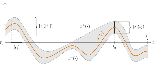
A tube is defined over a temporal t-domain \([t_0,t_f]\) as an envelope of trajectories that are defined over the same t-domain. We speak about an envelope as it may exist trajectories enclosed in the tube that are not solutions of our problem.

In this library, a tube \([x](\cdot):[t_0,t_f]\rightarrow\mathbb{IR}\) is an interval of two trajectories \([\underline{x}(\cdot),\overline{x}(\cdot)]\) such that \(\forall t\in[t_0,t_f]\), \(\underline{x}(t)\leqslant\overline{x}(t)\). We also consider empty tubes that depict an absence of solutions, denoted \(\varnothing(\cdot)\). A trajectory \(x(\cdot)\) belongs to the tube \(\left[x\right](\cdot)\) if \(\forall t\in[t_0,t_f], x\left(t\right)\in\left[x\right]\left(t\right)\).

../../_images/tube_def.png — Fig. 8 Illustration a one-dimensional tube enclosing a trajectory \(x^*(\cdot)\) plotted in orange. The figure shows two interval evaluations: \([x]([t_1])\) and \([x](t_2)\).

Note

Important: we assume that all the tubes and/or the trajectories involved in a given resolution process share the same t-domain \([t_0,t_f]\).

Slices 

In Codac, tubes are implemented as lists of slices.

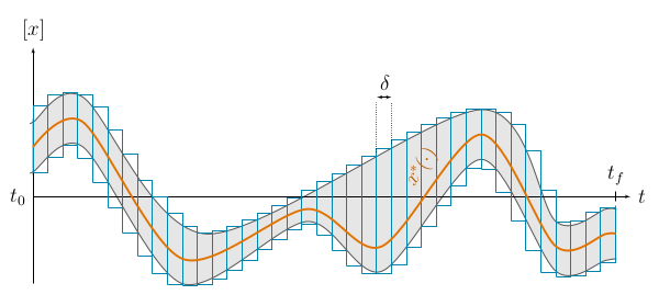
More precisely, a tube \([x](\cdot)\) with a sampling time \(\delta>0\) is implemented as a box-valued function which is constant for all \(t\) inside intervals \([k\delta,k\delta+\delta]\), \(k\in\mathbb{N}\).

The box \([k\delta,k\delta+\delta]\times\left[x\right]\left(t_{k}\right)\), with \(t_{k}\in[k\delta,k\delta+\delta]\), is called the \(k\)-th slice of the tube \([x](\cdot)\) and is denoted by \([\![x]\!]^{(k)}\).

../../_images/02_tube_slices.png — Fig. 9 A tube \([x](\cdot)\) represented by a set of \(\delta\)-width slices. This implementation can be used to enclose signals such as \(x^*(\cdot)\).

Added in version 2.0: Custom discretization of tubes is now at hand, they can be made of slices that are not all defined with the same sampling time \(\delta\).

This implementation takes rigorously into account floating point precision when building a tube. Further computations involving \([x](\cdot)\) will be implicitly based on its slices, thus keeping a reliable outer approximation of the solution set.

Creating tubes 

The vocabulary for tubes involves two notions:

the t-domain, that represents the temporal domain \([t_0,t_f]\)
the codomain, that represents the set of feasible values of the tube \([x]([t_0,t_f])\)

To create a Tube with a constant codomain:

tdomain = Interval(0,10)

# One-slice tubes:
x1 = Tube(tdomain)                               # [0,10]→[-∞,∞]
x2 = Tube(tdomain, Interval(0,2))                # [0,10]→[0,2]

# 100-slices tubes:
dt = 0.1
x3 = Tube(tdomain, dt, Interval(0,2))            # [0,10]→[0,2]
x4 = Tube(tdomain, dt, Interval(0,oo))           # [0,10]→[0,∞]

Interval tdomain(0,10);

// One-slice tubes:
Tube x1(tdomain);                                // [0,10]→[-∞,∞]
Tube x2(tdomain, Interval(0,2));                 // [0,10]→[0,2]

// 100-slices tubes:
float dt = 0.1;
Tube x3(tdomain, dt, Interval(0,2));             // [0,10]→[0,2]
Tube x4(tdomain, dt, Interval(0,oo));            // [0,10]→[0,∞]

The dt variable defines the temporal width of the slices. Note that it is also possible to create slices of different width; this will be explained afterwards.

To create a copy of a tube with the same time discretization, use:

x5 = Tube(x4)                    # identical tube (100 slices, [0,10]→[0,∞])
x5.set(Interval(5))              # 100 slices, same timestep, but [0,10]→[5]

Tube x5(x4);                     // identical tube (100 slices, [0,10]→[0,∞])
x5.set(Interval(5.));            // 100 slices, same timestep, but [0,10]→[5]

As tubes are intervals of trajectories, a Tube can be defined from Trajectory objects:

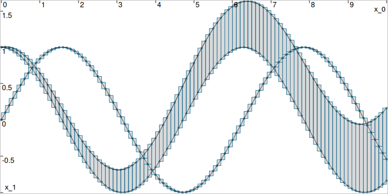
traj = TrajectoryVector(tdomain, TFunction("(sin(t) ; cos(t) ; cos(t)+t/10)"))

x8 = Tube(traj[0], dt)           # 100 slices tube enclosing sin(t)
x9 = Tube(traj[1], traj[2], dt)  # 100 slices tube defined as [cos(t),cos(t)+t/10]

TrajectoryVector traj(tdomain, TFunction("(sin(t) ; cos(t) ; cos(t)+t/10)"));

Tube x8(traj[0], dt);            // 100 slices tube enclosing sin(t)
Tube x9(traj[1], traj[2], dt);   // 100 slices tube defined as [cos(t),cos(t)+t/10]

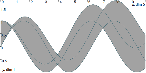
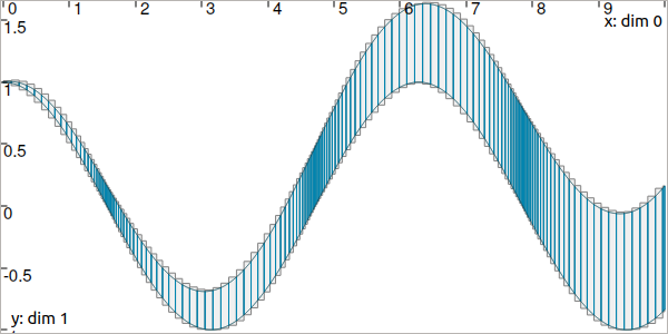
../../_images/interval_trajs.png — Fig. 10 Result of tubes \([x_8](t)=[\sin(t),\sin(t)]\), \([x_9](t)=[\cos(t),\cos(t)+\frac{t}{10}]\), made of 100 slices.

It is also possible to create a tube from a thick function, where the uncertainty is explicitly set in the formula:

dt = 0.01
x10 = Tube(tdomain, dt, \
           TFunction("-abs(cos(t)+t/5)+(t/2)*[-0.1,0.1]"))

dt = 0.01;
Tube x10(tdomain, dt,
         TFunction("-abs(cos(t)+t/5)+(t/2)*[-0.1,0.1]"));

../../_images/02_tube_fnc.png — Fig. 11 Result of tube \([x_{10}](\cdot)\) made of 1000 slices.

Finally, as tube is an envelope (union) of trajectories, the following operations are allowed:

f = TFunction("(cos(t) ; cos(t)+t/10 ; sin(t)+t/10 ; sin(t))") # 4d temporal function
traj = TrajectoryVector(tdomain, f) # 4d trajectory defined over [0,10]

# 1d tube [x](·) defined as a union of the 4 trajectories
x = Tube(traj[0], dt) | traj[1] | traj[2] | traj[3]

TFunction f("(cos(t) ; cos(t)+t/10 ; sin(t)+t/10 ; sin(t))"); // 4d temporal function
TrajectoryVector traj(tdomain, f); // 4d trajectory defined over [0,10]

// 1d tube [x](·) defined as a union of the 4 trajectories
Tube x = Tube(traj[0], dt) | traj[1] | traj[2] | traj[3];

Which produces:

The vector case 

The extension to the vector case is the class TubeVector, allowing to create tubes \([\mathbf{x}](\cdot):[t_0,t_f]\to\mathbb{IR}^n\).

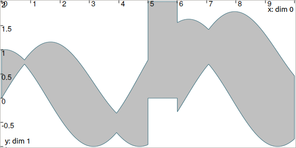
The following example

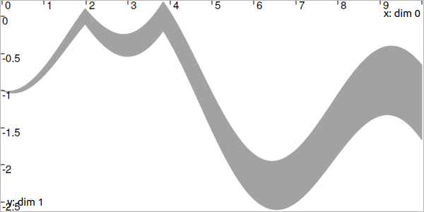
# TubeVector from a formula; the function's output is two-dimensional
x = TubeVector(tdomain, dt, \
               TFunction("(sin(sqrt(t)+((t-5)^2)*[-0.01,0.01]) ; \
                          cos(t)+sin(t/0.2)*[-0.1,0.1])"))

// TubeVector from a formula; the function's output is two-dimensional
TubeVector x(tdomain, dt,
             TFunction("(sin(sqrt(t)+((t-5)^2)*[-0.01,0.01]) ; \
                        cos(t)+sin(t/0.2)*[-0.1,0.1])"));

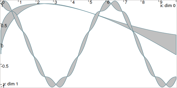
produces (each dimension displayed on the same figure):

Added in version 3.0.10: The definition of a TubeVector can also be done from a list. The above example could be written as:

# TubeVector as a list of scalar tubes
x = TubeVector([ \
    Tube(tdomain, dt, TFunction("(sin(sqrt(t)+((t-5)^2)*[-0.01,0.01]))")), \
    Tube(tdomain, dt, TFunction("cos(t)+sin(t/0.2)*[-0.1,0.1]")) \
  ])

// TubeVector as a list of scalar tubes
TubeVector x({
    Tube(tdomain, dt, TFunction("(sin(sqrt(t)+((t-5)^2)*[-0.01,0.01]))")),
    Tube(tdomain, dt, TFunction("cos(t)+sin(t/0.2)*[-0.1,0.1]"))
  });

As for Vector and IntervalVector objects, a Tube component of a TubeVector is available by reference with []. Vector operations are also at hand:

Return type	Code	Meaning
`int`	`x.size()`	number of dimensions of the tube vector
–	`x.resize(n)`	adds or removes dimensions
`TubeVector`	`x.subvector(start_id, end_id)`	extracts a subvector from `x`
–	`x.put(start_id, v)`	puts a subvector at `start_id`

Evaluations 

Once created, several evaluations of the tubes can be made, as for trajectories.

Accessing values with ()

x(6.)                            # evaluation of [x](·) at 6
x(Interval(5,6))                 # evaluation of [x](·) over [5,6]
x.codomain()                     # envelope of values

x(6.)                            // evaluation of [x](·) at 6
x(Interval(5.,6.))               // evaluation of [x](·) over [5,6]
x.codomain()                     // envelope of values

Inversion of tubes

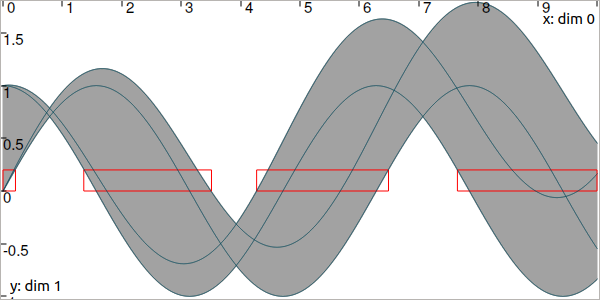
The inversion of a tube \([x](\cdot)\), denoted \([x]^{-1}([y])\), returns the set \([t]\) enclosing the preimages of \([y]\). The invert() method returns the squared-union of these subsets, or the set of solutions within a vector of Interval objects. The following example returns the different subsets of the inversion \([x]^{-1}([0,0.2])\) projected in red in next figure:

v_t = []
x.invert(Interval(0,0.2), v_t, tdomain)   # inversion
# tdomain is a temporal subset over which the inversion is performed

for t in v_t:
  tbox = IntervalVector([t,[0,0.2]])
  fig.draw_box(tbox, "red")      # boxes display

vector<Interval> v_t;            // vector of preimages
x.invert(Interval(0.,0.2), v_t, tdomain); // inversion
// tdomain is a temporal subset over which the inversion is performed

for(auto& t : v_t)
{
  IntervalVector tbox = {t,{0.,0.2}};
  fig.draw_box(tbox, "red");     // boxes display
}

Operations on sets 

Set operations are available for Tube and TubeVector objects. In the following table, if \([x](\cdot)\) is a tube object, \(z(\cdot)\) is a trajectory.

Return type	Code	Meaning, \(\forall t\in[t_0,t_f]\)
`bool`	`x==y`	\([x](t)=[y](t)\)
`bool`	`x!=y`	\([x](t)\neq [y](t)\)
`bool`	`x.is_empty()`	\([x](t)=\varnothing\)
`bool`	`x.is_subset(y)`	\([x](t)\subseteq [y](t)\)
`bool`	`x.is_strict_subset(y)`	\([x](t)\subseteq [y](t)\wedge [x](t)\neq [y](t)\)
`bool`	`x.is_superset(y)`	\([x](t)\supseteq [y](t)\)
`bool`	`x.is_strict_superset(y)`	\([x](t)\supseteq [y](t)\wedge [x](t)\neq [y](t)\)
`BoolInterval`	`x.contains(z)`	\(z(t)\in [x](t)\)
`bool`	`x.overlaps(y)`	\([x](t)\cap [y](t)\neq\varnothing\)

The contains() method

Testing if a tube \([x](\cdot)\) contains a solution \(z(\cdot)\) may lead to uncertainties. Indeed, the reliable representation of a Trajectory may lead to some wrapping effect, and so this contains test may not be able to conclude. Therefore, the contains() method returns a BoolInterval value. Its values can be either YES, NO or MAYBE. The MAYBE case is rare but may appear due to the numerical representation of a trajectory. In practice, this may happen if the thin envelope of \(z(\cdot)\) overlaps a boundary of the tube \([x](\cdot)\).

In addition of these test functions, operations on sets are available:

Code	Meaning, \(\forall t\in[t_0,t_f]\)
`x&y`	\([x](t)\cap [y](t)\)
`x\|y`	\([x](t)\sqcup[y](t)\)
`x.set_empty()`	\([x](t)\leftarrow \varnothing\)
`x=y`	\([x](t)\leftarrow [y](t)\)
`x&=y`	\([x](t)\leftarrow ([x](t)\cap [y](t))\)
`x\|=y`	\([x](t)\leftarrow ([x](t)\sqcup[y](t))\)

Finally, one can also access properties of the sets. First for Tube:

Return type	Code	Meaning
`Trajectory`	`x.diam()`	diameters of the tube as a trajectory, \(d(\cdot)=\overline{x}(\cdot)-\underline{x}(\cdot)\)
`double`	`x.max_diam()`	maximal diameter
`double`	`x.volume()`	the volume (surface) of the tube
`Tube`	`x.inflate(eps)`	a Tube with the same midtraj and radius increased by `eps`

Then for TubeVector:

Return type	Code	Meaning
`TrajectoryVector`	`x.diam()`	diameters of the tube as a trajectory, \(\mathbf{d}(\cdot)=\overline{\mathbf{x}}(\cdot)-\underline{\mathbf{x}}(\cdot)\)
`Vector`	`x.max_diam()`	maximal diameter
`Trajectory`	`x.diag()`	approximated trajectory: list of diagonals of each slice
`double`	`x.volume()`	the volume of the tube
`TubeVector`	`x.inflate(eps)`	new tube: same midtraj, each dimension increased by `eps`

The diam() methods

These methods are used to evaluate the thickness of a Tube or a TubeVector. They are mainly used for display purposes, for instance for displaying a tube with a color function depending on its thickness.

However, without derivative knowledge, and because the tube is made of boxed slices, the trajectory will be discontinuous and so the returned object will not reliably represent the actual diameters.

The diag() methods

It holds the same of the diag() methods.

Classical operations on sets are applicable on tubes. We recall that the tubes and trajectories have to share the same t-domain for these operations.

x4 = (x1 | x2) & x3

Tube x4 = (x1 | x2) & x3;

The same for mathematical functions:

x2 = abs(x1)
x3 = cos(x1) + sqrt(x2 + pow(x1, Interval(2,3)))

Tube x2 = abs(x1);
Tube x3 = cos(x1) + sqrt(x2 + pow(x1, Interval(2,3)));

The following functions can be used:

Code	Meaning
`sqr(x)`	\([x](\cdot)^2\)
`sqrt(x)`	\(\sqrt{[x](\cdot)}\)
`pow(x,n)`	\([x](\cdot)^n\)
`pow(x,y)`	\([x](\cdot)^{[y]} = e^{[y]\log([x](\cdot))}\)
`root(x,n)`	\(\sqrt[n]{[x](\cdot)}\)
`exp(x)`	\(\exp([x](\cdot))\)
`log(x)`	\(\log([x](\cdot))\)
`cos(x)`	\(\cos([x](\cdot))\)
`sin(x)`	\(\sin([x](\cdot))\)
`tan(x)`	\(\tan([x](\cdot))\)
`acos(x)`	\(\textrm{acos}([x](\cdot))\)
`asin(x)`	\(\textrm{asin}([x](\cdot))\)
`atan(x)`	\(\textrm{atan}([x](\cdot))\)
`atan2(y,x)`	\(\textrm{atan2}([y](\cdot),[x](\cdot))\) \(\textrm{atan2}([y],[x](\cdot))\) \(\textrm{atan2}([y](\cdot),[x])\)

Integral computations 

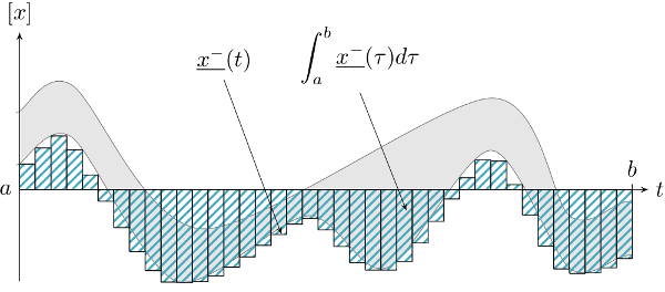
Reliable integral computations are available on tubes.

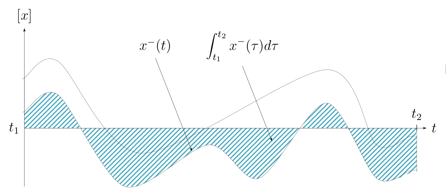
../../_images/tube_integ_inf.png — Fig. 12 Hatched part depicts the lower bound of \(\displaystyle\int_{a}^{b}[x](\tau)d\tau\).

The computation is reliable because it stands on the tube’s slices. The result is an outer approximation of the integral of the tube represented by these slices:

../../_images/tube_lb_integral_slices.png — Fig. 13 Outer approximation of the lower bound of \(\int_{a}^{b}[x](\tau)d\tau\).

Computation of the tube primitive \([p](\cdot)=\int_{0}^{\cdot}[x](\tau)d\tau\):

p = x.primitive()

Tube p = x.primitive();

Computation of the interval-integral \([s]=\int_{0}^{[t]}[x](\tau)d\tau\):

t = Interval(...)
s = x.integral(t)

Interval t(...);
Interval s = x.integral(t);

Computation of \([s]=\int_{[t_1]}^{[t_2]}[x](\tau)d\tau\):

t1 = Interval(...)
t2 = Interval(...)
s = x.integral(t1, t2)

Interval t1(...), t2(...);
Interval s = x.integral(t1, t2);

Also, a decomposition of the interval-integral of \([x](\cdot)=[x^-(\cdot),x^+(\cdot)]\) with \([s^-]=\int_{[t_1]}^{[t_2]}x^-(\tau)d\tau\) and \([s^+]=\int_{[t_1]}^{[t_2]}x^+(\tau)d\tau\) is computable by:

t1 = Interval(...)
t2 = Interval(...)
s = x.partial_integral(t1, t2)
# s[0] is [s^-]
# s[1] is [s^+]

Interval t1, t2;
pair<Interval,Interval> s;
s = x.partial_integral(t1, t2);
// s.first is [s^-]
// s.second is [s^+]

Note: \([s]=[s^-]\sqcup[s^+]\).

Updating values 

The set() methods allow various updates on tubes. For instance:

x.set(Interval(0,2), Interval(5,6)) # then [x]([5,6])=[0,2]

x.set(Interval(0.,2.), Interval(5.,6.)); // then [x]([5,6])=[0,2]

produces:

Warning

Be careful when updating a tube without the use of dedicated contractors. Tube discretization has to be kept in mind whenever an update is performed for some input \(t\). For reliable operations, please see the contractors section.

Sampling and t-domain 

The following methods are related to t-domains and slices structure:

Return type	Code	Meaning
`Interval`	`x.tdomain()`	temporal domain \([t_0,t_f]\) (t-domain)
–	`x.shift_tdomain(a)`	shifts the t-domain to \([t_0+a,t_f+a]\)
`bool`	`same_slicing(x, y)`	tests if `x` and `y` have the same slicing (static)
–	`x.sample(t)`	samples the tube at \(t\) (adds a slice)
–	`x.sample(y)`	samples `x` so that it shares the sampling of tube `y`
–	`x.remove_gate(t)`	removes the sampling at \(t\), if it exists

The sample() methods

Custom sampling of tubes is available. The sample(t) method allows to cut a slice defined over \(t\) into two slices on each side of \(t\). If \(t\) already separates two slices (if it corresponds to a gate), then nothing is changed.

Fig. 14 Example of custom slicing of a tube.

Next pages will present reliable operators to reduce the range of the presented domains (intervals, boxes, tubes) in a reliable way and according to the constraints defining a problem.

Technical documentation

See the C++ API documentation of this class: