Lesson C: Static range-and-bearing localization

In this lessson, we still focus on the perception of landmarks clearly identified: each observation is related to a known position. The problem is similar to the localization of the previous lesson, but now we also consider the bearing, i.e. the angular position of the rock with respect to the heading of the robot.

We will see how to handle this constraint. From this example, we will understand the principles of decomposition of constraints and the polar equations.

Content of this lesson

• Lesson C: Static range-and-bearing localization

  • Formalism

  • Decomposition of constraints

  • Optimality of contractors

  • The polar constraint

  • Initialization

  • State estimation

Formalism

For the moment, the map is made of one landmark. The localization problem corresponds to the following observation function:

\[\mathbf{y}=\mathbf{g}\big(\mathbf{x}\big)\]

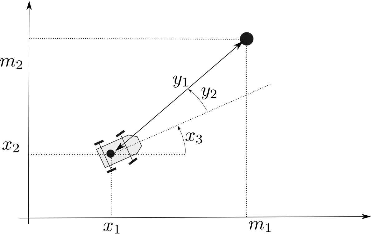
where \(\mathbf{x}\) is the unknown state vector: the robot is located at \(\left(x_{1},x_{2}\right)^\intercal\) with a heading \(x_{3}\). The output measurement vector is \(\mathbf{y}\), made of the range \(y_{1}\) and the bearing \(y_{2}\), as illustrated by the figure. It is assumed that the measurement is bounded: \(\mathbf{y}\in\left[\mathbf{y}\right]\), contrary to \(\mathbf{x}\) that is completely unknown: \(\mathbf{x}\in[\mathbf{x}]=[-\infty,\infty]^2\). We say that \([\mathbf{x}]\) is an unbounded set.

Often, the observation equation also appears in the following implicit form:

\[\mathbf{g}\big(\mathbf{x},\mathbf{y}\big)=\mathbf{0}.\]

In our range-and-bearing case, the observation equation is then defined as:

\[\begin{split}\mathbf{g}(\mathbf{x},\mathbf{y})=\left(\begin{array}{c} x_{1}+y_{1}\cdot\cos\left(x_{3}+y_{2}\right)-m_1\\ x_{2}+y_{1}\cdot\sin\left(x_{3}+y_{2}\right)-m_2 \end{array}\right),\end{split}\]

with \(\mathbf{m}\), the 2d position of the landmark.

Note that in a range-only case where the robot only measures the distance \(y\) to the landmark, we obtain the following relation:

\[g(\mathbf{x},y)=\left(x_{1}-m_1\right)^{2}+\left(x_{2}-m_2\right)^{2}-y^{2}.\]

In the more general case, the observation function \(\mathbf{g}\) is uncertain, or more precisely, it depends on some parameters that are not exactly known. For instance, the position of the landmark, denoted by the 2d vector \(\mathbf{m}\), may be uncertain. It can even be completely unknown if the landmark is not identified; this will be the case in the next lesson.

The related observation equation can be written as:

\[\mathbf{g}\big(\mathbf{x},\mathbf{y},\mathbf{m}\big)=\mathbf{0}.\]

In a set-membership approach, the uncertainties related to the state \(\mathbf{x}\), the measurement \(\mathbf{y}\) and the landmark \(\mathbf{m}\) will be implicitly represented by interval-vectors (boxes): \(\mathbf{x}\in[\mathbf{x}]\), \(\mathbf{y}\in[\mathbf{y}]\) and \(\mathbf{m}\in[\mathbf{m}]\).

We will solve this problem using the constraint programming approach.

Decomposition of constraints

Problems involving complex equations can be broken down into a set of primitive constraints. Here, primitive means that the constraints cannot be decomposed anymore. For instance, in a range-only localization problem (see Lessons A and B), the observation constraint \(\mathcal{L}_{\textrm{dist}}\) can be broken down into:

\[\begin{split}\mathcal{L}_{\textrm{dist}}: y=\sqrt{\left(x_1-m_1\right)^2+\left(x_2-m_2\right)^2} \Longleftrightarrow \left\{\begin{array}{rcll} a & = & x_1-m_1 & \big(\mathcal{L}_{-}\big)\\ b & = & x_2-m_2 & \big(\mathcal{L}_{-}\big)\\ c & = & a^2 & \big(\mathcal{L}_{(\cdot)^2}\big)\\ d & = & b^2 & \big(\mathcal{L}_{(\cdot)^2}\big)\\ e & = & c+d & \big(\mathcal{L}_{+}\big)\\ y & = & \sqrt{e} & \big(\mathcal{L}_{\sqrt{\cdot}}\big) \end{array}\right.\end{split}\]

where \(a,b,\dots,e\) are intermediate variables used for the decomposition. This constitutes a network made of the \(\mathcal{L}_{-}\), \(\mathcal{L}_{+}\), \(\mathcal{L}_{(\cdot)^2}\), and \(\mathcal{L}_{\sqrt{\cdot}}\) elementary constraints.

The library (more precisely: the IBEX library) provides a way to automatically make this decomposition, select already existing elementary contractors such as \(\mathcal{C}_{+}\), \(\mathcal{C}_{(\cdot)^2}\), \(\mathcal{C}_{\sqrt{\cdot}}\) and build the complex contractor modeling the constraint \(\mathcal{L}_{\textrm{dist}}\).

This was implicitly done in the previous Lesson A with:

Python

C++

ctc_dist = CtcFunction(Function("x[2]", "b[2]", "y",
    "sqrt((x[0]-b[0])^2+(x[1]-b[1]))-y"))

CtcFunction ctc_dist(Function("x[2]", "b[2]", "y",
    "sqrt((x[0]-b[0])^2+(x[1]-b[1]))-y"));

Optimality of contractors

Depending on the properties of the equation, the resulting contractor can be optimal. It means that the contracted box will perfectly enclose the set of feasible solutions without pessimism. This enables an efficient resolution.

In other cases, for instance because of dependencies between the variables, the resulting operator may not be optimal. For instance, looking at the equation depicting the above problem of range-and-bearing localization, the formula

\[\begin{split}\mathbf{g}(\mathbf{x},\mathbf{y})=\left(\begin{array}{c} x_{1}+y_{1}\cdot\cos\left(x_{3}+y_{2}\right)-m_1\\ x_{2}+y_{1}\cdot\sin\left(x_{3}+y_{2}\right)-m_2 \end{array}\right).\end{split}\]

could be implemented by

Python

C++

ctc_g = CtcFunction(Function("x[3]", "y[2]", "m[2]",
  "(x[0]+y[0]*cos(x[2]+y[1])-m[0] ; x[1]+y[0]*sin(x[2]+y[1])-m[1])"))

CtcFunction ctc_g(Function("x[3]", "y[2]", "m[2]",
  "(x[0]+y[0]*cos(x[2]+y[1])-m[0] ; x[1]+y[0]*sin(x[2]+y[1])-m[1])"));

However, this involves a multi-occurrence of variables which leads to pessimism. For instance, the sum \((x_3+y_2)\) appears twice in functions \(\cos\) and \(\sin\), which is hardly handled by a classical decomposition.

We may instead use a dedicated contractor that deals with the polar constraint, appearing in the above function \(\mathbf{g}\). This will allow us to avoid multi-occurrences and then, pessimism.

The polar constraint

The range-and-bearing problem is usually related to the polar constraint that links Cartesian coordinates to polar ones. This constraint is often encountered in robotics and it is important to be able to deal with it in an optimal way.

This simple and elementary constraint is expressed by:

\[\begin{split}\mathcal{L}_\textrm{polar}\big(d_1,d_2,\rho,\theta\big):~~~\mathbf{d}=\rho\cdot\left(\begin{array}{c} \cos(\theta)\\ \sin(\theta) \end{array}\right),\end{split}\]

where \(\rho\) and \(\theta\) are respectively the radial and angular coordinates.

It is elementary in the sense that it cannot be decomposed anymore without losing its optimality. In addition, a dedicated contractor already exists to deal with it: the CtcPolar.

Technical documentation

The CtcPolar page of the user manual provides more details about the contractor CtcPolar and the related publication.

This constraint appears in the expression of \(\mathbf{g}\).

Exercise

C.1. On a sheet of paper, write a decomposition of function \(\mathbf{g}\) that involves \(\mathcal{L}_\textrm{polar}\), other constraints and intermediate variables.

See the solution

Initialization

A robot depicted by the state \(\mathbf{x}=\left(2,1,\pi/6\right)^\intercal\) is perceiving a landmark \(\mathbf{m}=\left(5,6.2\right)^\intercal\) at a range \(y_1=6\) and a bearing \(y_2=\pi/6\). We assume that the position of the robot is not known and that the uncertainties related to the measurement and the landmark are:

• Measurement. For \(y_1\): \([-0.3,0.3]\), for \(y_2\): \([-0.1,0.1]\).

• Landmark. For each component of the 2d dimension: \([-0.2,0.2]\).

Exercise

C.2. Create a new project (Python or C++) and create the vectors x_truth, y_truth, m_truth representing the actual but unknown values of \(\mathbf{x}=\left(2,1,\pi/6\right)^\intercal\), \(\mathbf{y}=\left(6,\pi/6\right)^\intercal\) and \(\mathbf{m}=\left(5,6.2\right)^\intercal\).

Python

C++

# We recall that in Python, a mathematical vector (not an IntervalVector)
# can be represented with native objects, for instance:

x_truth = (2,1,math.pi/6) # actual state vector (pose)

// We recall that in C++, we can use the Vector class for
// representing mathematical vectors. For instance:

Vector x_truth({2.,1.,M_PI/6}); // actual state vector (pose)

C.3. Create the bounded sets related to the state, the measurement and the landmark position: \([\mathbf{x}]\in\mathbb{IR}^3\), \([\mathbf{y}]\in\mathbb{IR}^2\), \([\mathbf{m}]\in\mathbb{IR}^2\). We can for instance use the .inflate(float radius) method on intervals or boxes. The heading of the robot is assumed precisely known (for instance thanks to a compass); the actual heading \(x_3\) is represented by x_truth[2].

C.4. Display the vehicle and the landmark with:

Python

C++

beginDrawing()

fig_map = VIBesFigMap("Map")
fig_map.set_properties(100,100,500,500)
fig_map.axis_limits(0,7,0,7)
fig_map.draw_vehicle(x_truth, size=1)
fig_map.draw_box(m, "red")
fig_map.draw_box(x.subvector(0,1)) # does not display anything if unbounded
fig_map.show()

endDrawing()

vibes::beginDrawing();

VIBesFigMap fig_map("Map");
fig_map.set_properties(100,100,500,500);
fig_map.axis_limits(0,7,0,7);
fig_map.draw_vehicle(x_truth, 1);
fig_map.draw_box(m, "red");
fig_map.draw_box(x.subvector(0,1)); // does not display anything if unbounded
fig_map.show();

vibes::endDrawing();

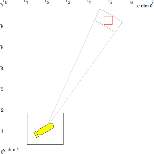
C.5. Display the range-and-bearing measurement with its uncertainties. For this, we will use the fig_map.draw_pie(x,y,interval_rho,interval_theta) to display a portion of a ring \([\rho]\times[\theta]\) centered on \((x,y)^\intercal\). Here, we add in \([\theta]\) the robot heading \(x_3\) and the bounded bearing \([y_2]\).

You should obtain this figure:

Fig. 29 On this figure, we also draw the origin of the measurement (in light gray). This can be done with:

draw_pie(x, y, (Interval(0.1)|interval_rho), interval_theta, "lightGray")

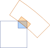
As one can see, intervals are not limited to axis-aligned boxes: we sometimes perform rotational mapping to better fit the set to represent. This polar constraint is a case in point.

State estimation

We will implement the decomposition of Question C.1 using the ContractorNetwork, that will manage the constraint propagation for us.

Exercise

The following must be made before the graphical part.

C.6. Create the contractors related to the decomposition of Question C.1.

• The contractor \(\mathcal{C}_\textrm{polar}\) is given by the class CtcPolar. Note that you do not need to create an object of this class, since one is already instantiated in the library (it is named ctc.polar in Python, ctc::polar in C++).

• The other contractors can be built with several CtcFunction objects, as we did in the previous Lessons A and B. We recall that these constraints have to be expressed in the form \(f(\mathbf{x})=0\). See more.

C.7. Create a ContractorNetwork (CN) to solve the problem by adding the contractors and the domains from the decomposition.

We recall that adding a contractor is made with:

Python

C++

cn = ContractorNetwork()
cn.add(<ctc_object>, [<dom1>,<dom2>,...])

ContractorNetwork cn;
cn.add(<ctc_object>, {<dom1>,<dom2>,...});

C.8. Create the intermediate variables introduced in Question C.1. They are Interval and IntervalVector objects, as for the other variables.

Note that the intermediate variables do not have to be initialized with prior values.

C.9. Use cn.contract() to solve the problem. You should obtain this figure:

The black box \([\mathbf{x}]\) cumulates all the uncertainties of the problem:

• uncertainties of the measurement

• uncertainties of the position of the landmark

If we remove the uncertainties related to the measurement \([\mathbf{y}]\), then the width of \([\mathbf{x}]\) should be exactly the same as the one of \([\mathbf{m}]\), because we used optimal contractors. The width of a box is given by the .diam() method.