See also
This manual refers to Codac v1, but a new v2 implementation is currently in progress… an update of this manual will be available soon. See more.
Introduction
Codac is a library providing tools for constraint programming over reals and trajectories. It has many applications in state estimation or robot localization.
Constraint programming
Codac is designed to deal with static and dynamical systems that are usually encountered in robotics. It stands on constraint programming: a paradigm in which the properties of a solution to be found (e.g. the pose of a robot, the location of a landmark) are stated by constraints coming from the equations of the problem.
Then, a solver performs constraint propagation on the variables and provides a reliable set of feasible solutions corresponding to the considered problem. In this approach, the user concentrates on what is the problem instead of how to solve it, thus leaving the computer dealing with the how. The strength of this declarative paradigm lies in its simpleness, as it allows one to describe a complex problem without requiring the knowledge of resolution tools coming with specific parameters to choose.
The following figure presents a conceptual view of a constraint propagation.
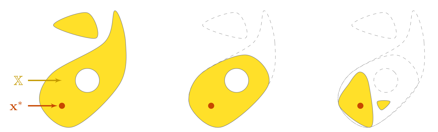
Fig. 1 In this theoretical view, a domain \(\mathbb{X}\) depicted in yellow is known to enclose a solution \(\mathbf{x}^*\) pictured by a red dot and consistent with two constraints \(\mathcal{L}_1\) and \(\mathcal{L}_2\). The estimation of \(\mathbf{x}^*\) consists in reducing \(\mathbb{X}\) while satisfying \(\mathcal{L}_1\) and \(\mathcal{L}_2\). After the propagation process, the set of feasible solutions has been reduced by removing vectors that were not consistent with the constraints: we obtain a finer approximation of \(\mathbf{x}^*\).
Variables
The unknown solutions of a system are reals \(x\), vectors \(\mathbf{x}\), or in the dynamic case: so-called trajectories denoted by \(x(\cdot)\), or \(\mathbf{x}(\cdot)\) in the vector case.
Dot notation \((\cdot)\)
Note that in the literature, the dot notation \((\cdot)\) may be used to represent the independent system variable (time). This notation may be chosen in order to clearly distinguish a whole trajectory \(\mathbf{x}(\cdot):\mathbb{R}\to\mathbb{R}^n\) from a local evaluation: \(\mathbf{x}(t)\in\mathbb{R}^n\). Indeed, the time \(t\) may also be a variable to be estimated.
In the constraint programming approach, the estimation of a variable consists in computing its reliable enclosure set, defined here as an interval of values. The obtained set is said reliable: the resolution guarantees that no solution can be lost during the solving process, according to the equations defining the problem. In other words, a variable \(x\) to be estimated will surely be enclosed in the resulting set \([x]\).
Domains
As depicted in the figure, a variable is known to be enclosed in some domain \(\mathbb{X}\) on which we will apply constraints. In Codac, the domains are represented by the following sets:
for reals \(x\), domains are intervals \([x]\);
for vectors \(\mathbf{x}\), we define boxes \([\mathbf{x}]\);
for trajectories \(x(\cdot)\), we introduce tubes \([x](\cdot)\).
Constraints
The approach consists in defining the problem as a set of constraints. They usually come from state equations, numerical models, or measurements. In mobile robotics, we usually have to deal with:
non-linear functions: \(x_3=\cos\big(x_1+\exp(x_2)\big)\)
differential equations: \(\dot{x}(\cdot)=f\big(x(\cdot),u(\cdot)\big)\)
temporal delays: \(x(t)=y(t-\tau)\)
time uncertainties: \(x(t)=y\), with \(t\in[t]\)
etc.
The aim of Codac is to easily deal with these constraints in order to eventually characterize sets of variables compliant with the defined rules. Each constraint comes from equations or measurements. And each constraint will be applied by means of an operator called contractor.
Contractors
Contractors are operators designed to reduce domains without losing any solution consistent with the related constraint. In Codac, the contractors act on intervals, boxes and tubes.
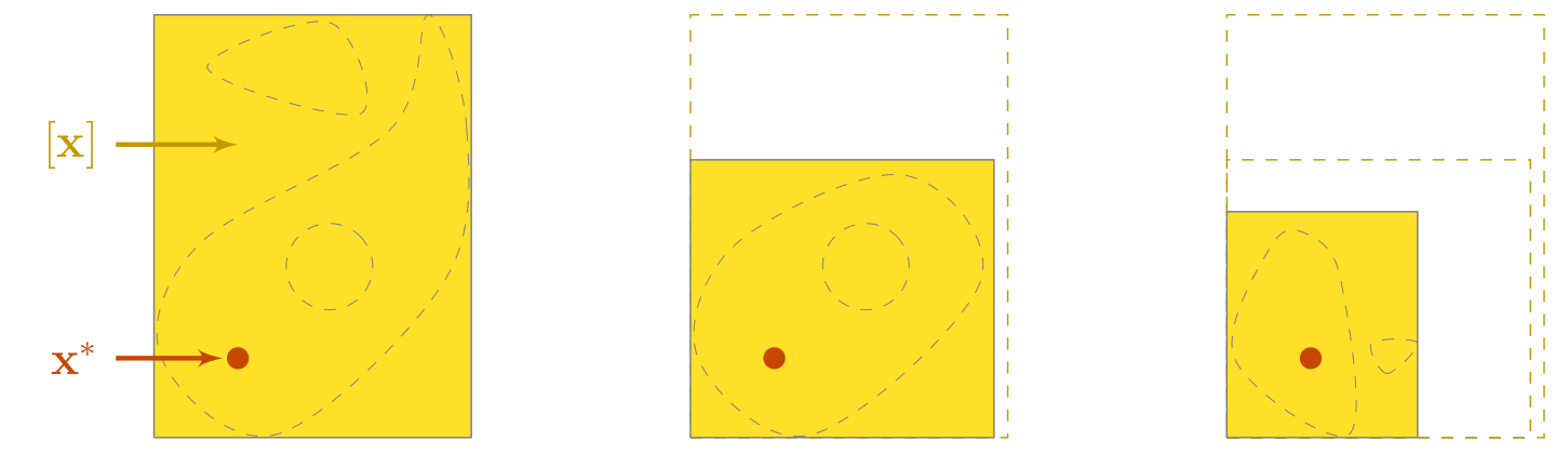
Fig. 2 Implementation of the constraints \(\mathcal{L}_1\) and \(\mathcal{L}_2\) of the previous figure by means of respective contractors \(\mathcal{C}_1\) and \(\mathcal{C}_2\). On this theoretical example, the domain \(\mathbb{X}\) is now a subset of a box \([\mathbf{x}]\), easily representable and contractible.
Codac already provides a catalog a contractors that one can use to deal with many applications. New contractors can also be designed and embedded in this framework without difficulty.
Constraint programming vs probabilistic methods
The approach does differ from probabilistic methods in regards of the nature of the estimated solution. Probabilistic methods compute a punctual potential solution – for instance a vector – while in set-membership ones, it is the set of all feasible solutions that is evaluated, and thus an infinity of potential solutions.
Another main distinction lies in the way things are computed: with set-membership methods, estimations are not randomly performed. Computations are deterministic: given a set of parameters or inputs, algorithms will always output the same result.
Reliable outputs
One of the advantages of this set-membership approach is the reliable outputs that are obtained. By reliable, we mean that all sources of uncertainties are taken into account, including:
model parameter uncertainties
measurement noise
uncertainties related to time discretization
linearization truncations
approximation of real numbers by floating-point values
The outcomes are intervals and tubes that are guaranteed to contain the solutions of the system. This is well suited for proof purposes as we always consider worst-case possibilities when delineating the boundaries of the solution sets.
The main drawback however, is that we may obtain large sets that may not be useful to characterize the solutions of the problem. We call this pessimism. This can be overcome by reformulating some constraints or by using bisections on sets.
The Codac library
The API of Codac can be broken down into three layers:
an extended intervals and tubes calculator
a catalog of contractors and separators for dynamical systems and mobile robotics
a system solver called Contractor Network
Each usage corresponds to a different layer and each layer is built on top of the previous one. This structure is similar to the one of IBEX, but dedicated to dynamical systems and robotic applications.
Codac has been designed by robotic researchers but provides a generic solver that has broader applications in guaranteed integration or parameter estimation.
What about the IBEX library?
The IBEX library is a C++ software for constraint processing over real numbers. As for Codac, it stands on Constraint Programming but focuses on static contexts, providing reliable algorithms for handling non-linear constraints.
It also proposes various tools such as the IbexSolve and IbexOpt plugins that are dedicated to system solving and optimization, and come both with a default black-box solver and global optimizer for immediate usage.
Codac is built upon IBEX and uses the elementary components of this library such as interval objects, arithmetic implementations, or contractors for static constraints. More precisely, Codac extends the contractor programming framework of IBEX to the dynamical case, introduces trajectories and tubes objects, gathers new contractors and separators together, and provides another kind of solver for heterogeneous systems made of both static and dynamical constraints.
Even if IBEX does not appear in the several robotic applications presented in this manual, it is still possible to build complex static contractors with IBEX and use them in Codac. Hence, IBEX can be used as a powerful contractor factory for static systems.