See also

This manual refers to Codac v1, but a new v2 implementation is currently in progress… an update of this manual will be available soon. See more.

Trajectories (signals)

A trajectory \(x(\cdot):[t_0,t_f]\to\mathbb{R}\) is a set of real values defined over some temporal domain \([t_0,t_f]\), called t-domain. They are aimed at representing temporal evolutions.

There are two ways to define a trajectory:

• with some analytic formula, by using a TFunction object ;

• from a map of values.

Defining a trajectory from an analytic function

It must be emphasized that the mathematical functions mentioned here are not related to programming functions in C++ or Python.

A simple temporal function [1] can be defined and used for building a trajectory:

PythonC++

tdomain = Interval(0,10)                               # temporal domain: [t_0,t_f]
x = Trajectory(tdomain, TFunction("cos(t)+sin(2*t)"))  # defining x(·) as: t ↦ cos(t)+sin(2t)

Usual functions such as \(\cos\), \(\log\), etc. can be used to define a TFunction object. The convention used for these definitions is the one of IBEX (read more). Note that the system variable \(t\) is a predefined variable of TFunction objects, that does not appear in IBEX’s objects.

The evaluation of a trajectory at some time \(t\), for instance \(z=x(t)\), is performed with parentheses:

PythonC++

z = x(math.pi)                               # z = cos(π)+sin(2π) = -1

In this code, \(x(\cdot)\) is implemented from the expression \(t\mapsto\cos(t)+\sin(2t)\), and no numerical approximation is performed: the formula is embedded in the object and the representation is accurate. However, the evaluation of the trajectory may lead to numerical errors related to the approximation of real numbers by floating-point values. For instance, if we change the decimal precision in order to format floating-point values, and then print the value of z, we can see that the result is not exactly \(-1\):

PythonC++

from decimal import *

z = x(math.pi)                               # z = cos(π)+sin(2π) = -1
print(Decimal(z))
// Output:
// -1.0000000000000006661338147750939242541790008544921875

This is not only due to the approximation made on \(\pi\), that could be reliably handled by some \([\pi]\).

A reliable evaluation of \(x(\cdot)\) can be done by specifying \(t\) as a degenerate interval \([t]\). This produces an interval evaluation that is reliable: the output is also an interval that is guaranteed to contain the actual value despite floating-point uncertainties:

PythonC++

z = x(Interval.PI)                           # z = cos(π)+sin(2π) = -1
print(z)
// Output:
// [-1.000000000000002, -0.9999999999999991]

This also works for large temporal evaluations as long as \([t]\subseteq[t_0,t_f]\).

Defining a trajectory from a map of values

Another way to build \(x(\cdot)\) is to implement it as a map of discrete values. \(x(\cdot)\) is supposed to be continuous and so linear interpolation is performed between each value of the map. These trajectories are useful in case of actual data coming from sensors or numerical models. The following example provides a comparison between the two kinds of trajectory definitions:

PythonC++

# Trajectory from a formula
x = Trajectory(Interval(0,10), TFunction("cos(t)+sin(2*t)"))

# Trajectory from a map of values
values = {}
for t in np.arange(0., 10., 0.5):
  values[t] = np.cos(t)+np.sin(2*t)
y = Trajectory(values)

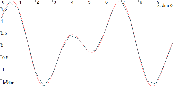
Fig. 3 In red, the trajectory defined from the analytical function. In blue, a trajectory made of 21 points with linear interpolation.

Note that when building a trajectory from a map, there is no need to specify the t-domain; it will be evaluated as the envelope of the keys of the map.

It is also possible to define a trajectory from an analytical function while representing it with a map of values. This can be necessary for various operations on trajectories that are not available for analytical definitions, such as arithmetic operations.

PythonC++

# Analytical definition but sampling representation with dt=0.5:
y_1 = Trajectory(Interval(0,10), TFunction("cos(t)+sin(2*t)"), 0.5)

# Same as before, in two steps. y_1 == y_2
y_2 = Trajectory(Interval(0,10), TFunction("cos(t)+sin(2*t)"))
y_2.sample(0.5)

The TFunction object is only used for the initialization. The resulting trajectory is only defined as a map of values.

Note

In Python: defining a trajectory from NumPy arrays

For instance, let us consider a \(n\times 1\) array and a \(n\times 3\) array for representing respectively time and 3d angles along time. The following allows to build a Trajectory for the third component:

data = np.load("data_angles.npz")
traj = Trajectory(data['t'][:],data['angles'][:,2])

Operations on trajectories

Once created, several evaluations of the trajectory can be made. For instance:

PythonC++

x.tdomain()        # temporal domain, returns [0, 10]
x.codomain()       # envelope of values, returns [-2,2]
x(6.)              # evaluation of x(·) at 6, returns 0.42..
x(Interval(5,6))   # evaluation of x(·) over [5,6], returns [-0.72..,0.42..]

Note that the items defining the trajectory (the map of values, or the function) are accessible from the object:

PythonC++

f = x.tfunction()                          # x(·) was defined from a formula
m = y.sampled_map()                        # y(·) was defined as a map of values

Other methods exist such as:

PythonC++

# Approximation of primitives:
y_prim = y.primitive()                     # when defined from a map of values
x_prim = x.primitive(0, 0.01)              # when defined from a function,
                                           # params are (x0,dt)
# Differentiations:
y_diff = y.diff()                          # finite differences on y(·)
x_diff = x.diff()                          # exact differentiation of x(·)

Note that the result of these methods is inaccurate on trajectories defined from a map. For trajectories built on analytic functions, the exact differentiation is performed and returned in the form of a trajectory defined by a TFunction too.

Finally, to add a point to a mapped trajectory, the following function can be used:

PythonC++

y.set(1, 4)                                # add the value y(4)=1

Other features and details can be found in the technical datasheet of the Trajectory class.

We summarize in the following table the operations supported for each kind of trajectory definition.

Operations	Analytical def.	Map of values def.
codomain()	✓	✓
evaluations	✓	✓
first_value()	✓	✓
last_value()	✓	✓
set()		✓
truncate_tdomain()	✓	✓
shift_tdomain()	✓	✓
sample()	✓	✓
make_continuous()		✓
primitive()	✓	✓
diff()	✓	✓
arithmetics (\(+,-,\cdot,/\))		✓

The vector case

The extension to the vector case is the class TrajectoryVector, allowing to create trajectories \(\mathbf{x}(\cdot):\mathbb{R}\to\mathbb{R}^n\). The use of the features presented above remain the same.

PythonC++

# Trajectory from a formula; the function's output is two-dimensional
x = TrajectoryVector(Interval(0,10), TFunction("(cos(t);sin(t))"))

# Trajectory from a map of values
y = TrajectoryVector(2)
for t in np.arange(0., 10., 0.6):
  y.set([np.cos(t),np.sin(t)], t)

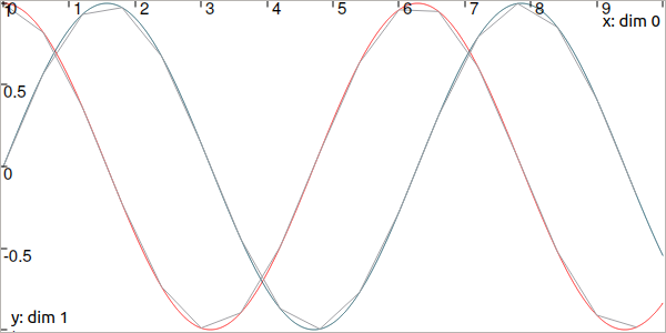
Fig. 4 In red and blue, the TrajectoryVector defined from the analytical function. In gray, the sampled one.

New in version 3.0.10: The definition of a TrajectoryVector can also be done from a list. The above example could be written as:

PythonC++

# TrajectoryVector as a list of scalar trajectories
x = TrajectoryVector([ \
    Trajectory(Interval(0,10), TFunction("cos(t)")), \
    Trajectory(Interval(0,10), TFunction("sin(t)")) \
  ])

Note that each component of a vector object (IntervalVector, TrajectoryVector, TubeVector) is available by reference:

PythonC++

x[1] = Trajectory(tdomain, TFunction("exp(t)"))
print(x[1])

Arithmetic on trajectories

In the same manner as for vectors, basic operations (\(+,-,\cdot,/\)) can be used on trajectories, together with usual mathematic functions: \(\cos\), \(\log\), etc. An example will explain it better.

Let us consider a robot following a Lissajous curve from \(t_0=0\) to \(t_f=5\):

PythonC++

tdomain = Interval(0,5)
x = TrajectoryVector(tdomain, TFunction("(2*cos(t) ; sin(2*t))"), 0.01)

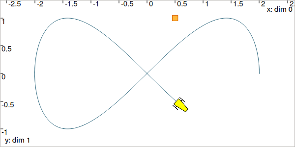
Fig. 5 Top view. The yellow robot follows a Lissajous curve forming an \(\infty\) symbol.

It continuously measures its distance to a landmark located at \((0.5,1)\). We compute the trajectory of distances by:

PythonC++

b = (0.5,1) # landmark's position
dist = sqrt(sqr(x[0]-b[0])+sqr(x[1]-b[1])) # simple operations between traj.

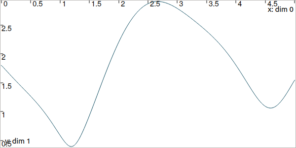
Fig. 6 Result of simulated range measurements: the dist trajectory object.

Random trajectories

As one can see, trajectories can be used to represent data. When it comes to consider some added noise, the RandTrajectory class may be useful.

PythonC++

# Random values in [-0.2,0.2] at each dt=0.01
n = RandTrajectory(tdomain, 0.01, Interval(-0.2,0.2))

dist += n # added noise (sum of trajectories)

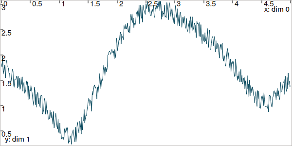
Fig. 7 Result of simulated range measurements with noise.

---

Next pages will present several methods to use tubes that are envelopes of trajectories: a reliable way to handle uncertainties over time.

Footnotes

[1]

In Codac, a codac::TFunction is the extension of IBEX’s Function objects, for the dynamical case (see more about IBEX’s functions).

Technical documentation

See the C++ API documentation of this class:

• Trajectory

• TrajectoryVector