See also

This manual refers to Codac v1, but a new v2 implementation is currently in progress… an update of this manual will be available soon. See more.

CtcEval: \(y_i=x(t_i)\)

\(y_i=x(t_i)\) is a constraint that links a value \(y_i\) to the evaluation of the trajectory \(x(\cdot)\) at time \(t_i\). A dedicated contractor \(\mathcal{C}_{\textrm{eval}}\) implements this constraint. One of its applications is the correction of the positions of a robot based on observations.

Definition

Important

\[\begin{split}\left.\begin{array}{r}y_i=x(t_i)\\\dot{x}(\cdot)=v(\cdot)\end{array}\right\} \longrightarrow \mathcal{C}_{\textrm{eval}}\big([t_i],[y_i],[x](\cdot),[v](\cdot)\big)\end{split}\]

PythonC++

ctc.eval.contract(ti, yi, x, v)

Prerequisite

The tubes \([x](\cdot)\) and \([v](\cdot)\) must share:

• the same slicing (same sampling of time)

• the same t-domain \([t_0,t_f]\)

• the same dimension of \([y_i]\) in the vector case

1d theoretical presentation

The \(\mathcal{C}_{\textrm{eval}}\) contractor aims at intersecting a tube \([x](\cdot)\) by the envelope of all trajectories compliant with the bounded observation \([t_i]\times[y_i]\). In other words, \([x](\cdot)\) will be contracted by the tube of all \(x(\cdot)\in[x](\cdot)\) going through the box \([t_i]\times[y_i]\), as shown in Fig. 22. Some trajectories may partially cross the box at some point over \([t_i]\): the contractor must take into account the feasible propagations during the intersection process. To this end, the knowledge of the derivative \(\dot{x}(\cdot)\) is required to depict the evolution of \(x(\cdot)\) over \([t_i]\).

The contractor is proposed in the most generic way; the derivative \(\dot{x}(\cdot)\) is also bounded within a tube denoted \([v](\cdot)\), thus allowing the \([x](\cdot)\) contraction even if the derivative signal is uncertain.

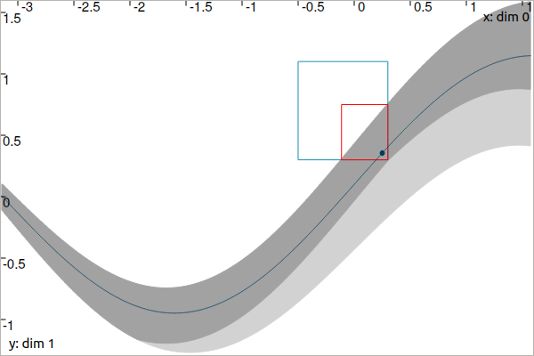
Fig. 22 Observation on a tube \([x](\cdot)\). A given measurement \(\mathbf{m}\in\mathbb{R}^{2}\), pictured by a black dot, is known to belong to the blue box \([t_i]\times[y_i]\). The sets are contracted by means of \(\mathcal{C}_{\textrm{eval}}\); the contracted part of the tube is depicted in light gray. Meanwhile, the bounded observation itself is contracted to \([t_i']\times[y_i']\) with \([t_i']\subseteq[t_i]\) and \([z_i']\subseteq[z_i]\). This is illustrated by the red box. The dark line is an example of a compliant trajectory. The derivative \(\dot{x}(\cdot)\), not represented here, is also enclosed within a tube.

The code leading to the contraction presented in this figure is:

PythonC++

dt = 0.01
tdomain = Interval(-math.pi, math.pi/2)

v = Tube(tdomain, dt, TFunction("cos(t)+[-0.1,0.1]")) # uncertain derivative (not displayed)
x = v.primitive() + Interval(-0.1, 0.1) # x is the primitive of v

# Bounded observation
ti = Interval(-0.5,0.3)
yi = Interval(0.3,1.1)

# Contraction
ctc_eval = CtcEval()
ctc_eval.contract(ti, yi, x, v)
# Note that we could use directly ctc.eval.contract(ti, yi, x, v)

Restrict the temporal propagation (save computation time)

\(\mathcal{C}_{\textrm{eval}}\) may contract the tube \([x](\cdot)\) and in this case, the contraction will be temporally propagated forward/backward in time from the \([t_i]\) t-domain. In Fig. 22, we can see that the contraction occurs over \([-1.9,t_f]\). The .enable_time_propag(false) method can be used to limit the contraction to the \([t_i]\) t-domain only. This is useful when dealing with several observations \([t_i]\times[z_i]\) on the same tube: it becomes faster to first perform all the local contractions over each \([t_i]\) and then smooth the tube only once with, for instance, the \(\mathcal{C}_{\frac{d}{dt}}\) contractor presented before.

For instance, we now consider three constraints on the tube:

PythonC++

ti = [Interval(-0.5,0.3), Interval(-0.6,0.8), Interval(-2.3,-2.2)]
yi = [Interval(0.3,1.1), Interval(-0.5,-0.4), Interval(-0.8,-0.7)]

Then we use the contractor configured for the limited contraction:

PythonC++

ctc_eval.enable_time_propag(False)

for i in range (0,3):
  ctc_eval.contract(ti[i], yi[i], x, v)

ctc.deriv.contract(x, v) # for smoothing the tube

for i in range (0,3): # for contracting the [ti]×[yi] boxes
  ctc_eval.contract(ti[i], yi[i], x, v)

The following animation presents the results before and after the \(\mathcal{C}_{\frac{d}{dt}}\) contraction:

Fixed point propagation

When dealing with several constraints on the same tube, a single application of \(\mathcal{C}_{\textrm{eval}}\) for each \([t_i]\times[y_i]\) may not provide optimal results. Indeed, \(\mathcal{C}_{\textrm{eval}}\) propagates an evaluation along the whole domain of \([x](\cdot)\) which may lead to new possible contractions. It is preferable to use an iterative method that applies all contractors indefinitely until they become ineffective on \([x](\cdot)\) and the \([t_i]\times[y_i]\)’s:

See also

The CN chapter for constraint propagation.

2d localization example

Contracting the tube

Let us come back to the Lissajous example of the previous page.

Assume now that we have no knowledge on \([\mathbf{x}](\cdot)\), except that the feasible trajectories go through the box \([\mathbf{b}]=[-0.73,-0.69]\times[0.64,0.68]\) at some time \(t\in[4.3,4.4]\).

The tube is contracted over \([t_0,t_f]\) with its uncertain derivative \([\mathbf{v}](\cdot)\) given by:

\[\begin{split}[\mathbf{v}](t) = \left(\begin{array}{c}-2\sin(t)\\2\cos(2t)\end{array}\right)+\left(\begin{array}{c} [-0.01,0.01]\\ [-0.01,0.01]\end{array}\right)\end{split}\]

PythonC++

dt = 0.01
tdomain = Interval(0,5)
# No initial knowledge on [x](·)
x = TubeVector(tdomain, dt, 2) # initialization with [-∞,∞]×[-∞,∞]

# New values for the temporal evaluation of [x](·)
t = Interval(4.3,4.4)
b = IntervalVector([[-0.73,-0.69],[0.64,0.68]])

# Uncertain derivative of [x](·)
v = TubeVector(tdomain, dt, TFunction("(-2*sin(t) ; 2*cos(2*t))"))
v.inflate(0.01)

# Contraction
ctc_eval = CtcEval()
ctc_eval.contract(t, b, x, v)
# Note that in this case, no contraction is performed on [t] and [b]
# Note also that we could use directly ctc.eval.contract(t, b, x, v)

The obtained tube is blue painted on the figure, the contraction to keep the trajectories going through \([\mathbf{b}]\) (red box) over \([t]=[4.3,4.4]\) is propagated over the whole t-domain:

Contracting the evaluation box

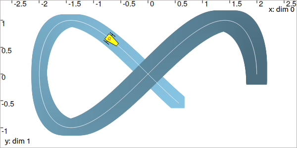
Assume now that we know the actual trajectory to be bounded within the tube:

\[\begin{split}[\mathbf{x}](t) = \left(\begin{array}{c}2\cos(t)\\\sin(2t)\end{array}\right)+\left(\begin{array}{c} [-0.05,0.05]\\ [-0.05,0.05]\end{array}\right)\end{split}\]

PythonC++

x = TubeVector(tdomain, dt, TFunction("(2*cos(t) ; sin(2*t))"))
x.inflate(0.05)

The tube is blue painted on the figure:

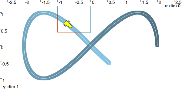
The yellow robot depicts an unknown position \(\mathbf{x}\) in the box \([-1,0]\times[0.4,1.2]\) at an unknown \(t\in[t_0,t_f]\). The \(\mathcal{C}_{\textrm{eval}}\) can be used to evaluate the position time and reduce the uncertainty on the possible positions.

PythonC++

t = Interval(0,oo) # new initialization
b = IntervalVector([[-1,0],[0.4,1.2]]) # (blue box on the figure)

ctc_eval.contract(t, b, x)

# [t] estimated to [4.15, 4.54]
# [b] contracted to ([-1, -0.29] ; [0.4, 0.95])  (red on the figure)

Related content

Related publication

Reliable non-linear state estimation involving time uncertainties

S. Rohou, L. Jaulin, L. Mihaylova, F. Le Bars, S. M. Veres

Automatica, 93:379–388, July 2018.

Download the paper

Technical documentation

See the C++ API documentation of this class.