See also

This manual refers to Codac v1, but a new v2 implementation is currently in progress… an update of this manual will be available soon. See more.

Lesson E: Hello tubes

Mobile robot motion is usually described by an evolution function \(\mathbf{f}\) involved in a differential equation. The interval state estimation then amounts to estimating the set of feasible trajectories that are solutions of this differential equation. The difficulty is to propagate the uncertainties in time, and to consider observations from asynchronous measurements in the same time. We will see that these difficulties are easily handled with constraint propagations on tubes.

Formalism

We now address the following problem:

\[\begin{split}\left\{ \begin{array}{lll} \dot{\mathbf{x}}(t)=\mathbf{f}\big(\mathbf{x}(t),\mathbf{u}(t)\big) & & \textrm{(evolution equation)}\\ \mathbf{y}(t)=\mathbf{g}\big(\mathbf{x}(t)\big) & & \textrm{(observation equation)} \end{array}\right.\end{split}\]

We recall that

• \(\mathbf{x}\in\mathbb{R}^n\) is the state vector

• \(\mathbf{u}\in\mathbb{R}^m\) is some input vector

• \(\mathbf{y}\in\mathbb{R}^p\) is a measurement

• and \(\mathbf{f}\), \(\mathbf{g}\) are respectively evolution and observation functions, possibly non-linear or uncertain

The \(\mathbf{x}\), \(\mathbf{u}\) and \(\mathbf{y}\) values continuously evolve with time. We will now handle them as trajectories.

What is a trajectory

A trajectory \(x(\cdot):[t_0,t_f]\to\mathbb{R}\) is a set of real values defined over some temporal domain \([t_0,t_f]\), called t-domain. They are aimed at representing temporal evolutions. We implement them with the Trajectory class (or the TrajectoryVector class for trajectories \(\mathbf{x}(\cdot):[t_0,t_f]\to\mathbb{R}^n\)).

These trajectories correspond to a new kind of variable in the constraint programming approach. We will consider them together with other values such as reals of vectors, as we did in the previous lessons.

New type of variables \(\implies\) new type of domain

Because we will deal with a new kind of variable (trajectories \(x(\cdot)\)), we also define a new type of domain to handle them with contractors: tubes \([x](\cdot)\).

A tube \([x](\cdot)\) is defined over a temporal t-domain \([t_0,t_f]\) as an envelope of trajectories that are defined over the same t-domain. We speak about an envelope as it may exist trajectories enclosed in the tube that are not solutions of our problem. A trajectory \(x(\cdot)\) belongs to the tube \(\left[x\right](\cdot)\) if \(\forall t\in[t_0,t_f], x\left(t\right)\in\left[x\right]\left(t\right)\).

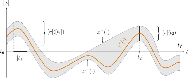
Fig. 36 Illustration a one-dimensional tube enclosing a trajectory \(x^*(\cdot)\) plotted in orange. The figure shows two interval evaluations: \([x]([t_1])\) and \([x](t_2)\).

Note

Important: we assume that all the tubes and/or the trajectories involved in a given resolution process share the same t-domain \([t_0,t_f]\).

The Tube class allows to create a tube. See more on: Tubes: sets of trajectories.

Using trajectories

Let us consider a robot following a Lissajous curve from \(t_0=0\) to \(t_f=5\). Its exact trajectory is given by:

\[\begin{split}\mathbf{x}^*(t) = \left(\begin{array}{c}2\cos(t)\\\sin(2t)\end{array}\right)\end{split}\]

The following code creates the actual (but unknown) trajectory \(\mathbf{x}^*(\cdot)\):

PythonC++

dt = 0.01
tdomain = Interval(0,5) # temporal domain [t0,tf]
actual_x = TrajectoryVector(tdomain, TFunction("(2*cos(t) ; sin(2*t))"), dt)

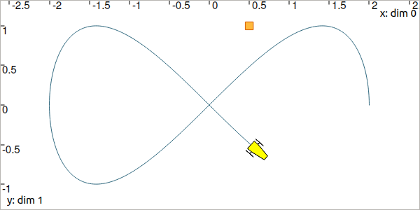
Fig. 37 Top view. The yellow robot follows a Lissajous curve forming an \(\infty\) symbol.

The TFunction object depicts a temporal function. It is similar to the Function objects we have seen previously, but the t variable is already defined. In this example, the output of the function is two-dimensional (defined with parenthesis).

The last argument dt converts the analytical function into a discretized signal with \(\delta=0.01\).

Exercise

E.1. In a new project, create the above trajectory \(\mathbf{x}^*(\cdot)\), named actual_x.

E.2. Create a landmark \(\mathbf{b}=(0.5,1)\).

E.3. In a VIBesFigMap figure, project the 2d trajectory in the view with the .add_trajectory() method. The arguments respectively refer to the object to display, its name in the view, the x-index component and the y-index component:

PythonC++

fig_map = VIBesFigMap("Map")
fig_map.set_properties(100, 100, 600, 300)
fig_map.add_trajectory(actual_x, "x*", 0, 1)
fig_map.add_beacon(b, 0.1)                    # 0.1: landmark width
fig_map.axis_limits(-2.5,2.5,-0.1,0.1, True)
fig_map.show(0.5)                             # argument is robot size

E.4. The robot continuously measures its distance to the landmark \(\mathbf{b}\).

Classical mathematical functions such as \(+\), \(\cos\), \(\exp\), \(\sqrt{\cdot}\), can be used on trajectories. Compute the distance signal actual_y between the robot and the landmark as one Trajectory object.

E.5. Display the actual_y trajectory in another dedicated view with a VIBesFigTube object:

PythonC++

fig_dist = VIBesFigTube("Distance to the landmark")
fig_dist.set_properties(100, 100, 600, 300)
fig_dist.add_trajectory(actual_y, "y*")
fig_dist.show()

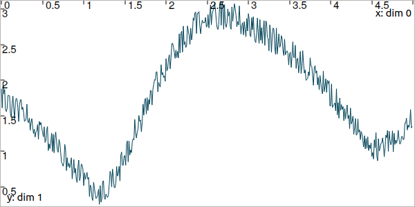
You should obtain this figure:

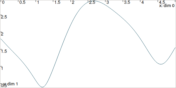
Fig. 38 Result of simulated range measurements: the actual_y trajectory object.

Enclosing the feasible trajectories of a robot

The state estimation will be done by enclosing the feasible trajectories in a tube submitted to contractors.

As for trajectories, tubes are defined over a t-domain \([t_0,t_f]\). A parameter \(\delta\) allows to numerically represent a tube as a set of temporal slices (we will use \(\delta\) = dt = 0.01).

We can build a tube from a temporal function, for instance:

PythonC++

dt = 0.01
tdomain = Interval(0,5)
a = Tube(tdomain, dt, TFunction("cos(t*2)"))

The same function can be used to express uncertainties with respect to time. For instance:

PythonC++

b = Tube(tdomain, dt, TFunction("cos(t*2)+abs(t*2-5)*[-0.1,0.1]"))

In the following figure, the tubes \([a](\cdot)\) and \([b](\cdot)\) are respectively drawn in dark gray and light gray.

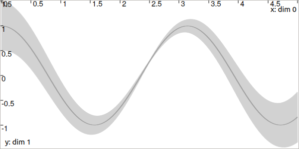
Fig. 39 The tube \([a](\cdot)\) has almost no uncertainty (thickness) over time (except the one due to its numerical representation) while the tube \([b](\cdot)\) in light gray has a thickness defined by \(|(2t-5)|\cdot[-0.1,0.1]\).

Tubes can also be built from trajectories. In this example, we could have defined \([a](\cdot)\) by:

PythonC++

actual_a = Trajectory(tdomain, TFunction("cos(t*2)"))
a = Tube(actual_a, dt) # [a](·) will wrap the trajectory

Exercise

E.6. Using the class TubeVector, create a 2d tube \([\mathbf{x}](\cdot)\) enclosing \(\mathbf{x}^*(\cdot)\). You may refer to the manual for more information on TubeVector.

E.7. Using the .inflate() method on x, inflate the tube so that \(\forall t,[\mathbf{x}](t)=\mathbf{x}^*(t)+[-0.2,0.2]\).

E.8. Display the tube in the previous figure with:

PythonC++

fig_map.add_tube(x, "x", 0, 1)
fig_map.show() # this method must be called to display the added objects

Is the actual trajectory \(\mathbf{x}^*(\cdot)\) enclosed in \([\mathbf{x}](\cdot)\) at any time?

E.9. Create a tube \([y](\cdot)\) for enclosing the actual trajectory \(y^{*}(\cdot)\) of distances between the robot and the landmark. For now, we will not consider uncertainties on \(y^{*}(\cdot)\). Therefore, the tube \([y](\cdot)\) should enclose \(y^{*}(\cdot)\) in a minimal way according to the discretization step dt. Note that all the tubes of this lesson have to share the same tdomain and dt parameters.

Involving tubes in a Contractor Network

We can now perform a localization based on range-only measurements. We will use again the distance contractor \(\mathcal{C}_{\textrm{dist}}\) developed in Lesson B: Static range-only localization but now in a dynamical context.

The contractors that act on boxes can be used on tubes without loss of generality and in a very transparent way. They will contract the tubes, slice by slice for each time in \([t_0,t_f]\).

For instance, one can contract three tubes \([a](\cdot)\), \([b](\cdot)\), \([c](\cdot)\), in order to be consistent with the \(\mathcal{L}_{+}\) constraint:

PythonC++

# a = Tube(...  (creating tubes)
# b = Tube(...
# c = Tube(...

# The constraint "x1+x2=x3" is equivalent to "x1+x2-x3=0":
ctc_add = CtcFunction(Function("x1", "x2", "x3", "x1+x2-x3"), Interval(0))

cn = ContractorNetwork()
cn.add(ctc_add, [a,b,c]) # the tubes are listed according to the constraint definition
cn.contract()

Exercise

We recall the problem:

\[\begin{split}\left\{ \begin{array}{lll} \dot{\mathbf{x}}(t)=\mathbf{f}\big(\mathbf{x}(t),\mathbf{u}(t)\big) & & \textrm{(evolution equation)}\\ \mathbf{y}(t)=\mathbf{g}\big(\mathbf{x}(t)\big) & & \textrm{(observation equation)} \end{array}\right.\end{split}\]

E.10. We first focus on the observation equation \(\mathbf{y}(t)=\mathbf{g}\big(\mathbf{x}(t)\big)\). Build a contractor network and contract the tube \([\mathbf{x}](\cdot)\) with the distance contractor, that expresses \(\mathbf{g}\). Note that this contractor is already defined in the library. You developed your own version as an exercise in Lesson A, but you can also use:

PythonC++

ctc.dist # object already created, as for ctc.polar

You should obtain something like this:

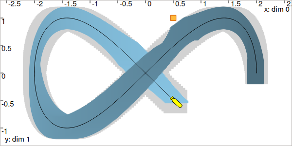
Fig. 40 Note: if you call again the .show() method after contracting the tube, the view will display the previous envelope of the tube in light gray, and the new contracted one in blue, as in the above figure. This helps to assess the contraction effect.

As one can see, the contraction is reliable: the actual trajectory (in dark blue) is kept in the tube. However, the contraction is not efficient. We need to also consider the differential equation \(\dot{\mathbf{x}}(t)=\mathbf{f}\big(\mathbf{x}(t),\mathbf{u}(t)\big)\).

Dealing with a differential equation

The equation \(\dot{\mathbf{x}}(t)=\mathbf{f}\big(\mathbf{x}(t),\mathbf{u}(t)\big)\) depicts the evolution of the robot. In this lesson, we assume that its actual speed \(\mathbf{v}^*(\cdot)\) is given in the absolute reference frame by:

\[\begin{split}\mathbf{v}^*(t) = \left(\begin{array}{c}-2\sin(t)\\2\cos(2t)\end{array}\right)\end{split}\]

Note that there is no difficulty to handle datasets instead of analytical functions: once the tube is defined (from functions or datasets), then the constraints will act on its bounds, in the same manner.

Then, the evolution equation amounts to \(\dot{\mathbf{x}}(t)=\mathbf{v}(t)\).

Exercise

E.11. Enclose \(\mathbf{v}^*(\cdot)\) in a tube \([\mathbf{v}]=\mathbf{v}^*(\cdot)+[-0.01,0.01]\).

E.12. A contractor exists to deal with the differential constraint:

\[\left.\begin{array}{r}\dot{\mathbf{x}}(\cdot)=\mathbf{v}(\cdot)\end{array}\right. \longrightarrow \mathcal{C}_{\frac{d}{dt}}\big([\mathbf{x}](\cdot),[\mathbf{v}](\cdot)\big)\]

It takes as input a tube \([\mathbf{x}](\cdot)\) and a tube containing the set of feasible derivatives: \([\mathbf{v}](\cdot)\). This will smooth \([\mathbf{x}](\cdot)\).

This contractor is also predefined in the library:

PythonC++

ctc.deriv # object already created, as for ctc.polar

Add this contractor to your Contractor Network.

You should obtain this result:

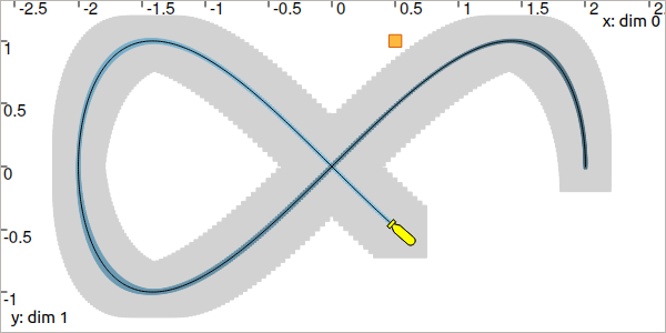
Fig. 41 The contraction is maximal when all the constraints are considered simultaneously.

(optional) Adding noise on the measurements

The RandTrajectory class allows to create a trajectory with random values.

PythonC++

# Random values in [-0.1,0.1] at each dt=0.01
n = RandTrajectory(tdomain, 0.01, Interval(-0.1,0.1))

Exercise

E.13. (optional) Add a noise, bounded by \([-0.05,0.05]\), to the distance trajectory:

E.14. (optional) What should be the uncertainties on \([y](\cdot)\) in order to reliably enclose the actual values despite the noise?

E.15. (optional) Compute the state estimation taking into account these errors.