CtcDeriv: \(\dot{x}(t)=v(t)\)

\(\dot{x}(t)=v(t)\) is the simplest differential constraint that binds a trajectory \(x(\cdot)\) to its derivative \(v(\cdot)\). The related contractor \(\mathcal{C}_{\frac{d}{dt}}\) allows contractions on the tube \([x](\cdot)\) to preserve only trajectories consistent with the derivatives enclosed in the tube \([v](\cdot)\).

Definition

Important

\[\left.\begin{array}{r}\dot{x}(\cdot)=v(\cdot)\end{array}\right. \longrightarrow \mathcal{C}_{\frac{d}{dt}}\big([x](\cdot),[v](\cdot)\big)\]

PythonC++

ctc.deriv.contract(x,v)

Prerequisite

The tubes \([x](\cdot)\) and \([v](\cdot)\) must share:

• the same slicing (same sampling of time)

• the same t-domain \([t_0,t_f]\)

• the same dimension in the vector case

Theoretical illustration

Here is an example of a consistency state reached with \(\mathcal{C}_{\frac{d}{dt}}\) over a set of trajectories and their feasible derivatives.

Let us consider two arbitrary tubes \([x](\cdot)\) and \([v](\cdot)\) and the constraint \(\dot{x}(t)=v(t)\).

PythonC++

dt = 0.01
tdomain = Interval(0., math.pi)

v = Tube(tdomain, dt, TFunction("sin(t+3.14+(3.14/2))/5+[-0.05,0.05]+(3.14-t)*[-0.01,0.01]"))
x = Tube(tdomain, dt, TFunction("[-0.05,0.05]+2+t*t*[-0.01,0.01]"))

The following images depict the tubes. The dark gray parts are the obtained tubes after the contraction performed by:

PythonC++

ctc_deriv = CtcDeriv()
ctc_deriv.contract(x,v)
# one could also directly use: ctc.deriv.contract(x,v)

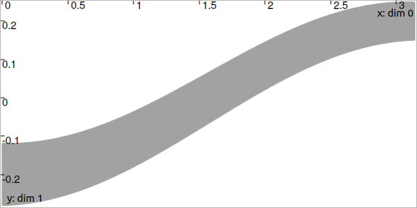
Fig. 20 The tube \([v](\cdot)\).

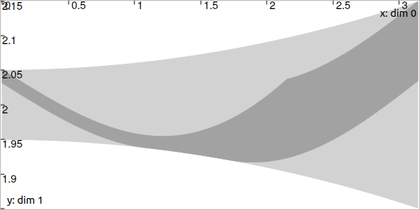
Fig. 21 The tube \([x](\cdot)\). The light-gray part has been contracted with \(\mathcal{C}_{\frac{d}{dt}}\).

Only \([x](\cdot)\) is contracted (it can be theoretically proved that \([v](\cdot)\) cannot be contracted when \([x](\cdot)\) is not a degenerate tube). Note that all the feasible derivatives in \([v](\cdot)\) are negative over \([0,1]\) and so the contraction of \([x](\cdot)\) preserves decreasing trajectories over this part of the domain. Similarly, \([v](\cdot)\) is positive over \([2,3]\) which corresponds to increasing trajectories kept in \([x](\cdot)\) after contraction.

Localization example

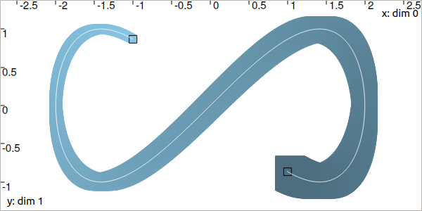
Let us consider another example with 2d tubes. We come back to the Lissajous example introduced to present the use of trajectories.

We assume that we have no knowledge on \([\mathbf{x}](\cdot)\), except that the feasible trajectories start from the initial box \([\mathbf{x}_0]\) at \(t_0\) and \([\mathbf{x}_f]\) at \(t_f\), black painted in the following figure.

PythonC++

dt = 0.01
tdomain = Interval(0,math.pi).inflate(math.pi/3)

# The unknown truth is given by:
x_truth = TrajectoryVector(tdomain, TFunction("(2*cos(t) ; sin(2*t))"))

# From the truth we build the initial and final conditions
# with some uncertainties (inflate)
x0 = IntervalVector(x_truth(tdomain.lb())).inflate(0.05)
xf = IntervalVector(x_truth(tdomain.ub())).inflate(0.05)

# No initial knowledge on [x](·)..
x = TubeVector(tdomain, dt, 2) # 2d tube defined over [t_0,t_f] with dt sampling

# ..except for initial and final conditions
x.set(x0, tdomain.lb())
x.set(xf, tdomain.ub())

The feasible derivatives are enclosed in \([\mathbf{v}](\cdot)\) given by:

\[\begin{split}[\mathbf{v}](t) = \left(\begin{array}{c}-2\sin(t)\\2\cos(2t)\end{array}\right)+\left(\begin{array}{c} [-0.02,0.02]\\ [-0.02,0.02]\end{array}\right)\end{split}\]

PythonC++

# Derivative of [x](·)
v = TubeVector(tdomain, dt, TFunction("(-2*sin(t) ; 2*cos(2*t))"))
v.inflate(0.02)

We can smooth the 2d tube \([\mathbf{x}](\cdot)\) in order to keep the envelope of trajectories starting in \([\mathbf{x}_0]\) at \(t_0\) and ending in \([\mathbf{x}_f]\) at \(t_f\). For this, we use the \(\mathcal{C}_{\frac{d}{dt}}\):

PythonC++

ctc.deriv.contract(x, v)

Which leads to:

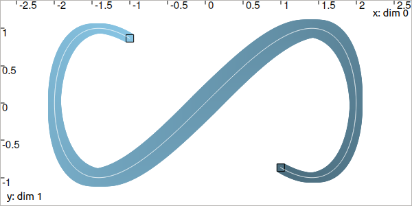
Note that the propagation happens in a temporal forward/backward way: from \(t_0\) to \(t_f\) as well as from \(t_f\) to \(t_0\). A third argument of the contract() method can be used to restrict the propagation way:

PythonC++

ctc.deriv.contract(x, v, TimePropag.BACKWARD) # or TimePropag.FORWARD

Which produces, for instance, backward contractions from \([\mathbf{x}_f]\) only (in light blue):

Related content

Related publication

Guaranteed computation of robot trajectories

S. Rohou, L. Jaulin, L. Mihaylova, F. Le Bars, S. M. Veres

Robotics and Autonomous Systems, 93:76–84, 2017.

Download the paper

Technical documentation

See the C++ API documentation of this class.