See also

This manual refers to Codac v1, but a new v2 implementation is currently in progress… an update of this manual will be available soon. See more.

Lesson B: Static range-only localization

We now have all the material to compute a solver for state estimation.

Problem statement

Our goal is to deal with the problem of localizing a robot of state \(\mathbf{x}\in\mathbb{R}^2\) that measures distances \(d^{k}\) from three landmarks \(\mathbf{b}^{k}\), \(k\in\{1,2,3\}\). We consider uncertainties on both the measurements and the location of the landmarks, which means that \(d^{k}\in[d^{k}]\) and \(\mathbf{b}^{k}\in[\mathbf{b}^{k}]\). For now, the robot does not move.

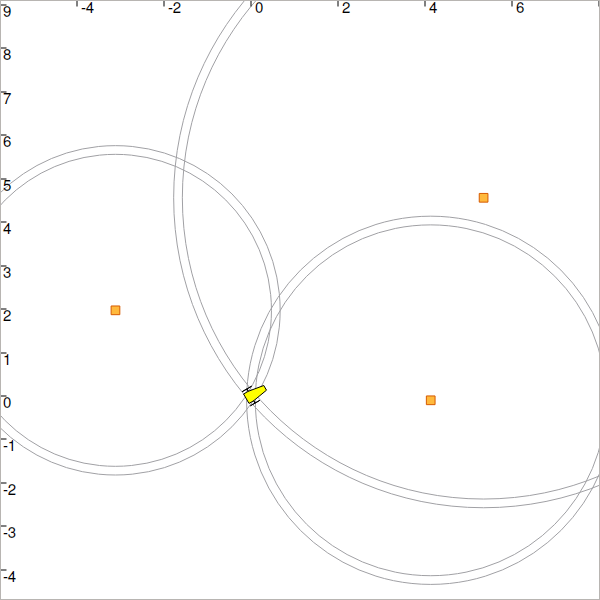
Fig. 27 The \(\mathbf{b}^{k}\) landmarks are depicted in orange while range-only measurements with bounded uncertainties are drawn by rings.

Our problem corresponds to the following Constraint Network:

\[\begin{split}\left\{ \begin{array}{l} \textrm{Variables:}~~ \mathbf{x}, \mathbf{b}^{1}, \mathbf{b}^{2}, \mathbf{b}^{3}, d^{1}, d^{2}, d^{3}\\ \textrm{Constraints:}~~ \\ -~ \mathcal{L}_{\textrm{dist}}^{1}\left(\mathbf{x},\mathbf{b}^{1},d^{1}\right) \\ -~ \mathcal{L}_{\textrm{dist}}^{2}\left(\mathbf{x},\mathbf{b}^{2},d^{2}\right) \\ -~ \mathcal{L}_{\textrm{dist}}^{3}\left(\mathbf{x},\mathbf{b}^{3},d^{3}\right) \\ \textrm{Domains:}~~ [\mathbf{x}], [\mathbf{b}^{1}], [\mathbf{b}^{2}], [\mathbf{b}^{3}], [d^{1}], [d^{2}], [d^{3}] \end{array}\right.\end{split}\]

This formalization can be seen in the literature and summarizes the problem in terms of variables, constraints on the variables, and domains for their sets of feasible values. As explained in the previous section, we will represent domains by means of intervals and boxes (interval vectors). In addition, constraints will be applied with contractors.

The \(\mathcal{L}_{\textrm{dist}}^{k}\) is the distance constraint from a landmark \(\mathbf{b}^{k}\). It links a measurement \(d^{k}\) to the state \(\mathbf{x}\) with:

\[\mathcal{L}_{\textrm{dist}}^{k}:~d^{k}=\sqrt{\left(x_1-b_1^{k}\right)^2+\left(x_2-b_2^{k}\right)^2}.\]

Solving the problem

The following code provides a simulation of random landmarks and related range-only measurements:

PythonC++

from codac import *
import math

# Truth (unknown pose)
x_truth = [0,0,math.pi/6] # (x,y,heading)

# Creating random map of landmarks
map_area = IntervalVector(2, [-8,8])
v_b = DataLoader.generate_landmarks_boxes(map_area, nb_landmarks = 3)

# The following function generates a set of [range]x[bearing] values
v_obs = DataLoader.generate_static_observations(x_truth, v_b, False)

# We keep range-only observations from v_obs, and add uncertainties
v_d = []
for obs in v_obs:
  d = obs[0].inflate(0.1) # adding uncertainties: [-0.1,0.1]
  v_d.append(d)

# Set of feasible positions for x: x ϵ [-∞,∞]×[-∞,∞]
x = IntervalVector(2) # this is equivalent to: IntervalVector([[-oo,oo],[-oo,oo]])

# ...

Finally, the graphical functions are given by:

PythonC++

# ...

beginDrawing()

fig = VIBesFigMap("Map")
fig.set_properties(50, 50, 600, 600)

for b in v_b:
  fig.add_beacon(b.mid(), 0.2)

for i in range(0,len(v_d)):
  fig.draw_ring(v_b[i][0].mid(), v_b[i][1].mid(), v_d[i], "gray")

fig.draw_vehicle(x_truth, size=0.7)
fig.draw_box(x) # estimated position
fig.show()

endDrawing()

Exercise

B.1. Before the code related to the graphical part, compute the state estimation of the robot by contracting the box \([\mathbf{x}]\) initialized to \([-\infty,\infty]^2\) with a Contractor Network:

• \([\mathbf{x}]\) represents the unknown 2d position of the robot

• v_d is the set of bounded measurements \(\{[d^{1}],[d^{2}],[d^{3}]\}\)

• v_b is the set of landmarks with bounded positions \(\{[\mathbf{b}^{1}],[\mathbf{b}^{2}],[\mathbf{b}^{3}]\}\)

For this, you can use the \(\mathcal{C}_{\textrm{dist}}\) contractor you defined in the previous section.

You should obtain a figure similar to this:

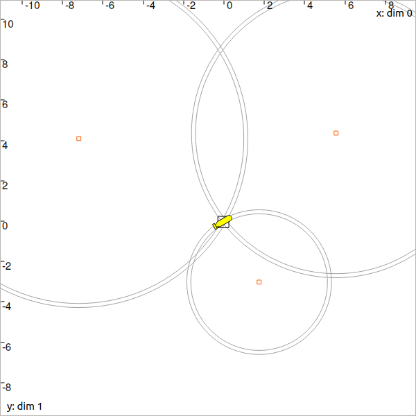
Fig. 28 Range-only localization: expected result. The black painted box represents the set of feasible positions for our robot.

Due to the randomness of the landmarks, the geometry is sometimes bad and does not allow an accurate contraction: symmetrical solutions are possible, and the box \([\mathbf{x}]\) encloses them all. You can execute the code several times to see how the geometry influences the result.

How does it work?

Combining the constraints

The Contractor Network you have defined managed the contractions provided by the three \(\mathcal{C}_{\textrm{dist}}\) contractors.

Each constraint alone would not allow a good contraction, since it would contract \([\mathbf{x}]\) to the box enclosing the circle corresponding to \(d^k\). It is the intersection of the three constraints that makes the approach powerful.

Fixed point resolution

There are dependencies between the constraints that all act on the same variable \(\mathbf{x}\). The Contractor Network has then made a fixed point resolution method for solving the problem.

When a \(\mathcal{C}_{\textrm{dist}}\) contractor reduces the box \([\mathbf{x}]\), it may raise new contraction possibilities coming from the other constraints. It becomes interesting to call again the previous contractors (start another iteration) in order to take benefit from any contraction. An iterative resolution process is then used, where the contractors are called until a fixed point has been reached. By fixed point we mean that none of the domains \([\mathbf{x}]\) and \([d^{k}]\) has been contracted during a complete iteration.

The following figure provides the synoptic of this state estimation, performed by the Contractor Network. In this example, constraints have been propagated over 7 iterations in a very short amount of time.

End of first step!

That’s about all for this first step!

Next lessons will introduce other concepts of constraint propagation. We will also see how to build our own contractor.