See also
This manual refers to Codac v1, but a new v2 implementation is currently in progress… an update of this manual will be available soon. See more.
Lesson A: Getting started with intervals and contractors
Now that Codac has been installed on your computer or usable online, we will get used to intervals, constraints and networks of contractors. This will allow you to perform the state estimation of a static robot between some landmarks by the end of Lesson B.
Start a new project
Start a new project as explained in:
Exercise
A.0. Check that it is displaying a tube in a graphical view and print the tube in the terminal using:
print(x)
cout << x << endl;
x
You should see the following output:
Tube [0, 10]↦([-1.448469806203122, 1.500000000000001]), 1000 slices
from codac import *

# .. next questions will be here
#include <codac.h>

using namespace std;
using namespace codac;

int main()
{
  // .. next questions will be here
}
import py.codac.*

% .. next questions will be here
Using intervals for handling uncertainties
The values involved in robotic problems will be represented by sets. This allows to hold in the very same structure both the value (a measurement, or a model parameter) together with the related uncertainty. Therefore, a measurement \(x\) will be handled by a set, more precisely an interval, denoted between brackets: \([x]\). \([x]\) is made of two real bounds, \(x^-\) and \(x^+\), and we say that a value \(x\in\mathbb{R}\) belongs to \([x]=[x^-,x^+]\) iff \(x^-\leqslant x\leqslant x^+\).
This can be extended to other types of values such as vectors, matrices or trajectories. Then,
reals \(x\) of \(\mathbb{R}\) will be enclosed in intervals: \([x]\)
vectors \(\mathbf{x}\) of \(\mathbb{R}^n\) will be enclosed in interval-vectors (also called boxes): \([\mathbf{x}]\)
later on, trajectories \(x(t)\) will belong to tubes: \([x](t)\)
The initial definition of the bounds of these sets will be done according to the amount of uncertainties we are considering. For measurements, we will rely on the datasheet of the sensor to define for instance that a measurement \(y\) will be represented by the interval \([y − 2\sigma, y + 2\sigma]\), where \(\sigma\) is the standard deviation coming from sensors specifications. In this case, we assume that the interval \([y]\) is guaranteed to contain the actual but unknown value with a 95% confidence rate.
The main advantage of this representation is that we will be able to apply lot of reliable operations on these sets while preserving the actual but unknown values. This means that we will never lose a feasible solution in the initial sets throughout the operations we will perform. This is done by performing the computations on the bounds of the sets. For instance, the difference of two intervals is also an interval defined by: \([x]-[y]=[x^--y^+,x^+-y^-]\). Mathematically, we can prove that \(\forall x\in[x]\) and \(\forall y\in[y]\), we have \((x-y)\in([x]-[y])\).
These simple operations on intervals can be extended to elementary functions such as \(\cos\), \(\exp\), \(\tan\), etc. It must be emphasized that there is no need to make linearizations when dealing with non-linear functions. Sometimes, when functions are monotonic, the computation is simple: \(\exp([x])=[\exp(x^-),\exp(x^+)]\). Otherwise, several algorithms and libraries exist to allow any mathematical operations on intervals such as \(\sin([x])\), \(\sqrt{([x])}\), etc.
The asset of reliability coming with interval analysis will help us to estimate difficult solutions and make proofs.
Hello Interval Analysis!
Codac is using C++/Python objects to represent intervals and boxes [1]:
Interval(lb, ub)will be used to create an interval \([x]=[\textrm{lb},\textrm{ub}]\). There exists predefined values for intervals. Here are some examples ofIntervalobjects:x = Interval() # [-∞,∞] (default value) x = Interval(0, 10) # [0,10] x = Interval(1, oo) # [1,∞] x = Interval(-oo,3) # [-∞,3] x = Interval.EMPTY_SET # ∅ # ...
Interval x;                                 // [-∞,∞] (default value)
Interval x(0, 10);                          // [0,10]
Interval x(1, oo);                          // [1,∞]
Interval x(-oo, 3);                         // [-∞,3]
Interval x = Interval::EMPTY_SET;           // ∅
// ...
IntervalVector(n)is used for \(n\)-d vectors of intervals, also called boxes.For instance:x = IntervalVector(2, [-1,3]) # creates [x]=[-1,3]×[-1,3]=[-1,3]^2 y = IntervalVector([[3,4],[4,6]]) # creates [y]= [3,4]×[4,6] z = IntervalVector(3, [0,oo]) # creates [z]=[0,∞]^3 w = IntervalVector(y) # creates a copy: [w]=[y] v = (0.42,0.42,0.42) # one vector (0.42;0.42;0.42) iv = IntervalVector(v) # creates one box that wraps v: # [0.42,0.42]×[0.42,0.42]×[0.42,0.42]
IntervalVector x(2, Interval(-1,3));        // creates [x]=[-1,3]×[-1,3]=[-1,3]^2
IntervalVector y{{3,4},{4,6}};              // creates [y]= [3,4]×[4,6]
IntervalVector z(3, Interval(0,oo));        // creates [z]=[0,∞]^3
IntervalVector w(y);                        // creates a copy: [w]=[y]

Vector v(3, 0.42);                          // one vector (0.42;0.42;0.42)
IntervalVector iv(v);                       // creates one box that wraps v:
                                            //   [0.42,0.42]×[0.42,0.42]×[0.42,0.42]
One can access vector components as we do classically:
x[1] = Interval(0,10) # updates to [x]=[-1,3]×[0,10]
x[1] = Interval(0,10); // updates to [x]=[-1,3]×[0,10]
Technical documentation
For full details about Interval and IntervalVector objects, please read the Intervals and boxes page of the user manual.
Exercise
A.1. Let us consider two intervals \([x]=[8,10]\) and \([y]=[1,2]\). Without coding the operation, what would be the result of \([x]/[y]\) (\([x]\) divided by \([y]\))? Remember that the result of this interval-division is also an interval enclosing all feasible divisions.
A.2. In your new project, compute and print the following simple operations on intervals:
Solutions are given below
\([-2,4]\cdot[1,3]\) [-6,12]
\([8,10]/[-1,0]\) [-∞,-8]
\([-2,4]\sqcup[6,7]\) with operator
|[-2,7]\(\max([2,7],[1,9])\) [2,9]
\(\max(\varnothing,[1,2])\) ∅
\(\cos([-\infty,\infty])\) [-1,1]
\([-1,4]^2\) with function
sqr()[0,16]\(([1,2]\cdot[-1,3]) + \max([1,6]\cap[5,7],[1,2])\) [3,12]
|), i.e., \([x]\sqcup[y] = [[x]\cup[y]]\).A.3. Create a 2d box \([\mathbf{y}]=[0,\pi]\times[-\pi/6,\pi/6]\) and print the result of \(|[\mathbf{y}]|\) with abs().
Hint
How to use \(\pi\)?
# In Python, you can use the math module:
import math
x = math.pi
// In C++, you can use <math.h>:
#include <math.h>
double x = M_PI;
Note that in this code, the variable x is not the exact \(\pi\)! Of course, the mathematical one cannot be represented in a computer. But with intervals, we can manage reliable representations of floating point numbers. See more.
Functions, \(f([x])\)
Custom functions can be used on sets. For instance, to compute:
a Function object can be created by Function("<var1>", "<var2>", ..., "<expr>") and then evaluated over the set \([x]\):
x = Interval(-2,2)
f = Function("x", "x^2+2*x-exp(x)")
y = f.eval(x)
Interval x(-2,2);
Function f("x", "x^2+2*x-exp(x)");
Interval y = f.eval(x);
The first arguments of the function (only one in the above example) are its input variables. The last argument is the expression of the output. The result is the set of images of all defined inputs through the function: \([f]([x])=[\{f(x)\mid x\in[x]\}]\).
We can also define vector input variables and access their components in the function definition:
f = Function("x[2]", "cos(x[0])^2+sin(x[1])^2") # the input x is a 2d vector
Function f("x[2]", "cos(x[0])^2+sin(x[1])^2"); // the input x is a 2d vector
Exercise
A.4. For our robotic applications, we often need to define the distance function \(g\):
where \(\mathbf{x}\in\mathbb{R}^2\) would represent for instance the 2d position of a robot, and \(\mathbf{b}\in\mathbb{R}^2\) the 2d location of some landmark. Create \(g\) and compute the interval distance \([d]\) between the boxes \([\mathbf{x}]=[0,0]\times[0,0]\) and \([\mathbf{b}]=[3,4]\times[2,3]\). Note that in the library, the .eval() of functions only takes one argument: we have to concatenate the boxes \([\mathbf{x}]\) and \([\mathbf{b}]\) into one 4d interval-vector \([\mathbf{c}]\) and then compute \(g([\mathbf{c}])\). The concatenation can be done with the cart_prod function, see an example here.
Print the result that you obtain for \([d]=g([\mathbf{x}],[\mathbf{b}])\).
Graphics
The graphical tool VIBes has been created to Visualize Intervals and BoxES. It is compatible with simple objects such as Interval and IntervalVector. Its features have been extended in the Codac library with objects such as VIBesFigMap.
Exercise
A.5. Create a view with:
beginDrawing()
fig = VIBesFigMap("Map")
fig.set_properties(50, 50, 400, 400) # position and size

# ... draw objects here

fig.show() # display all items of the figure
endDrawing()
vibes::beginDrawing();
VIBesFigMap fig("Map");
fig.set_properties(50, 50, 400, 400); // position and size

// ... draw objects here

fig.show(); // display all items of the figure
vibes::endDrawing();
.show() method, draw the boxes \([\mathbf{x}]\) and \([\mathbf{b}]\) with the fig.draw_box(..) method. The computed interval range \([d]\) can be displayed as a ring centered on \(\mathbf{x}=(0,0)\). The ring will contain the set of all positions that are \(d\)-distant from \(\mathbf{x}=(0,0)\), with \(d\in[d]\).To display each bound of the ring, you can use fig.draw_circle(x, y, rad) where x, y, rad are real values.
Hint
To access real bounds of an Interval object x, you can use the x.lb()/x.ub() methods for lower and upper bounds. This also works with IntervalVector, returning vector items.
.inflate(0.1) method on x.Technical documentation
For full details about graphical features, please read the The VIBes viewer page of the user manual.
Want to use colors? Here is an example you can try:
fig.draw_box(x, "red[yellow]") # red: edge color of the box, yellow: fill color
fig.draw_box(x, "red[yellow]"); // red: edge color of the box, yellow: fill color
Contractors, \(\mathcal{C}([x])\)
This was an initial overview of what is Interval Analysis. Now, we will introduce concepts from Constraint Programming and see how the two approaches can be coupled for solving problems.
In robotics, constraints are coming from the equations of the robot. They can be for instance the evolution function \(\mathbf{f}\) or the observation equation with \(\mathbf{g}\). In the case of SLAM, we may also define a constraint to express the inter-temporal relation between different states \(\mathbf{x}_1\), \(\mathbf{x}_2\) at times \(t_1\), \(t_2\), for instance when a landmark has been seen two times.
Now, we want to apply the constraints in order to solve our problem. In the Constraint Programming community, we apply constraints on domains that represent sets of feasible values. The previously mentioned sets (intervals, boxes, tubes) will be used as domains.
We will use contractors to implement constraints on sets. They are mathematical operators used to contract (reduce) a set, for instance a box, without losing any feasible solution. This way, contractors can be applied safely any time we want on our domains.
In Codac, the contractors are also defined by C++/Python objects and are prefixed with Ctc. For this lesson, we will use the CtcFunction class to define a contractor according to a function \(f\). Note that the resulting contractor will aim at solving a constraint in the form \(f(\mathbf{x})=0\). This contractor has to be instantiated from a Function object defining the constraint. For instance, the simple constraint \((x+y=a)\) is expressed as \(f(x,y,a)=x+y-a=0\), and can be implemented as a contractor \(\mathcal{C}_+\) with:
ctc_add = CtcFunction(Function("x", "y", "a", "x+y-a"))
CtcFunction ctc_add(Function("x", "y", "a", "x+y-a"));
Exercise
A.8. Define a contractor \(\mathcal{C}_\textrm{dist}\) related to the distance constraint between two 2d positions \(\mathbf{x}\) and \(\mathbf{b}\in\mathbb{R}^2\). We will use the distance function previously defined, but in the form \(f(\mathbf{x},\mathbf{b},d)=0\).
x = Interval(0,1)
y = Interval(-2,3)
a = Interval(1,20)

cn = ContractorNetwork()   # Creating a Contractor Network
cn.add(ctc_add, [x, y, a]) # Adding the C+ contractor to the network,
                           # applied on three domains listed between braces
cn.contract()

# The three domains are then contracted as:
# x=[0, 1], y=[0, 3], a=[1, 4]
Interval x(0,1), y(-2,3), a(1,20);

ContractorNetwork cn;       // Creating a Contractor Network
cn.add(ctc_add, {x, y, a}); // Adding the C+ contractor to the network,
                            // applied on three domains listed between braces
cn.contract();

// The three domains are then contracted as:
// x=[0, 1], y=[0, 3], a=[1, 4]
Note that one contractor can be added several times in the CN. This is useful to apply several constraints implemented by the same operator, on different sets of variables.
Exercise
\([d]=[7,8]\)
\([\mathbf{x}]=[0,0]^2\)
\([\mathbf{b}^1]=[1.5,2.5]\times[4,11]\)
\([\mathbf{b}^2]=[3,4]\times[4,6.5]\)
\([\mathbf{b}^3]=[5,7]\times[5.5,8]\)
We recall that the same \(\mathcal{C}_\textrm{dist}\) object can appear several times in the CN.
Draw the \([\mathbf{b}^i]\) boxes (.draw_box()) and \([d]\) (.draw_circle()) before and after the contractions, in order to assess the contracting effects.
You should obtain this figure:
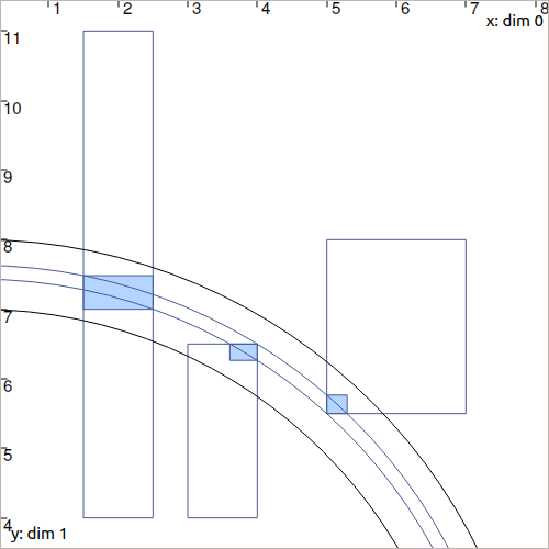
As you can see, the four domains have been contracted after the .contract() method: even the bounded range \([d]\) has been reduced thanks to the knowledge provided by the boxes. In Constraint Programming, we only define the constraints of the problem and let the resolution propagate the information as much as possible.
We now have all the material to compute a solver for state estimation in the next section.
Footnotes