See also

This manual refers to Codac v1, but a new v2 implementation is currently in progress… an update of this manual will be available soon. See more.

Lesson D: Building our own contractor

This lesson will extend the previous exercise by dealing with a data association problem together with localization: the landmarks perceived by the robot are now indistinguishable: they all look alike. The goal of this exercise is to develop our own contractor in order to solve the problem.

Introduction: indistinguishable landmarks

As before, our goal is to deal with the localization of a mobile robot for which a map of the environment is available.

It is assumed that:

• the map is static and made of point landmarks;

• the landmarks are indistinguishable (which was not the case before);

• the position of each landmark is known;

• the position of the robot is not known.

This problem often occurs when using sonars for localization, where it is difficult to distinguish a landmark from another. The challenge in this type of scenario is the difficulty of data associations, i.e. establishing feature correspondences between perceptions of landmarks and the map of these landmarks, known beforehand. This is especially the case of challenging underwater missions, for which one can reasonably assume that the detected landmarks cannot be distinguished from the other in sonar images. For instance, two different rocks may have the same aspect and dimension in the acquired images, as illustrated by the following figure.

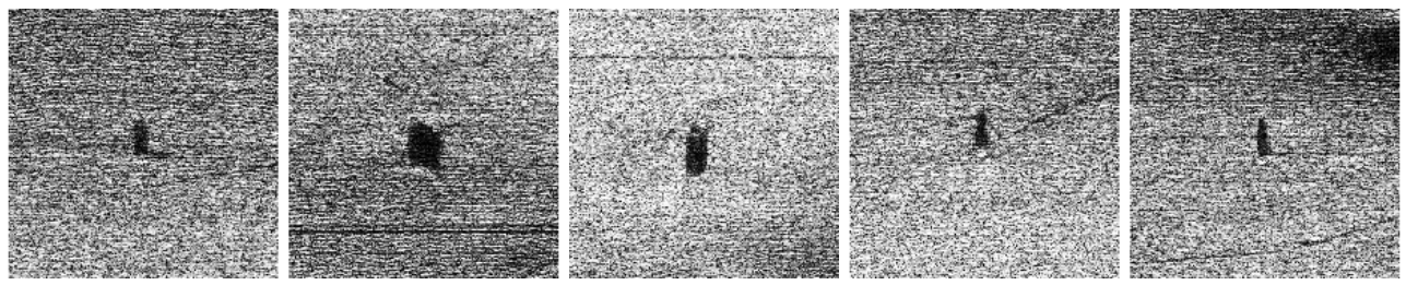
Fig. 30 Different underwater rocks perceived with one side-scan sonar. These observations are view-point dependent and the sonar images are noisy, which makes it difficult to distinguish one rock from another only from image processing. These sonar images have been collected by the Daurade robot (DGA-TN Brest, Shom, France) equipped with a Klein 5000 lateral sonar.

Due to these difficulties, we consider that we cannot compute reliable data associations that stand on image processing of the observations. We will rather consider the data association problem together with state estimation.

Data association: formalism

Up to now, we assumed that one perceived landmark was identified without ambiguity. However, when several landmarks \(\mathbf{m}_{1}\), \(\dots\), \(\mathbf{m}_{\ell}\) exist, the observation data may not be associated: we do not know to which landmark the measurement \(\mathbf{y}\) refers. We now consider several measurements denoted by \(\mathbf{y}^i\). Hence the observation constraint has the form:

\[\begin{split}\left\{ \begin{array}{l} \mathbf{g}\big(\mathbf{x},\mathbf{y}^{i},\mathbf{m}^{i}\big)=\mathbf{0},\\ \big(\mathbf{m}^{i}\in[\mathbf{m}_{1}]\big)\vee\dots\vee\big(\mathbf{m}^{i}\in[\mathbf{m}_{\ell}]\big), \end{array}\right.\end{split}\]

with \(\mathbf{m}^{i}\) the unidentified landmark of the observation \(\mathbf{y}^i\). The \(\vee\) notation expresses the logical disjunction or. Equivalently, the system can be expressed as:

\[\begin{split}\left\{ \begin{array}{l} \mathbf{g}\big(\mathbf{x},\mathbf{y}^{i},\mathbf{m}^{i}\big)=\mathbf{0},\\ \mathbf{m}^{i}\in\mathbb{M}=\left\{ [\mathbf{m}_{1}],\dots,[\mathbf{m}_{\ell}]\right\}, \end{array}\right.\end{split}\]

where \(\mathbb{M}\) is the bounded map of the environment: the set of all landmarks represented by their bounded positions. In other words, we do not know the right parameter vector \(\mathbf{m}_{1}\), \(\dots\), \(\mathbf{m}_{\ell}\) associated with the observation \(\mathbf{y}^i\). This is a problem of data association. The following figure illustrates \(\mathbb{M}\) with the difficulty to differentiate landmarks in underwater extents.

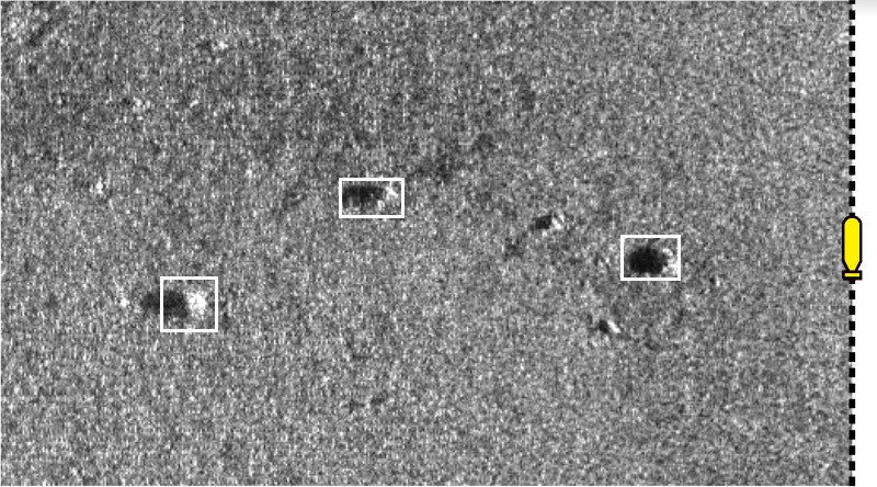
Fig. 31 The yellow robot, equipped with a side-scan sonar, perceives at port side some rocks \(\mathbf{m}^{i}\) lying on the seabed. The rocks, that can be used as landmarks, are assumed to belong to small georeferenced boxes \(\mathbb{M}\) enclosing uncertainties on their positions. The robot is currently not able to make any difference between the rocks, as it is typically the case in underwater extents when acoustic sensors are used to detect features.

In this exercise, the data association problem is solved together with state estimation, without image processing. The constraint \(\mathbf{g}\big(\mathbf{x},\mathbf{y}^{i},\mathbf{m}^{i}\big)=\mathbf{0}\) has been solved in Lesson C, it remains to deal with the constraint \(\mathbf{m}^{i}\in\mathbb{M}\). We will call it the constellation constraint.

The constellation constraint and its contractor

When solving a problem with a constraint propagation approach, we may not have the contractors at hand for dealing with all the involved constraints. In this lesson for instance, we assume that we do not have a contractor for dealing with this constellation constraint. The goal of the following exercise is to see how to build our own contractor. We will see that it is easy to extend our framework with new contractors, without loss of generality.

We now focus on the constellation constraint without relation with the other equations. The constraint is expressed by \(\mathcal{L}_{\mathbb{M}}\left(\mathbf{a}\right)~:~\mathbf{a}\in\mathbb{M}\).

Let us consider a constellation of \(\ell\) landmarks \(\mathbb{M}=\{[\mathbf{m}_{1}],\dots,[\mathbf{m}_{\ell}]\}\) of \(\mathbb{IR}^{2}\) and a box \([\mathbf{a}]\in\mathbb{IR}^2\). Our goal is to compute the smallest box containing \(\mathbb{M}\cap[\mathbf{a}]\). In other words, we want to contract the box \([\mathbf{a}]\) so that we only keep the best envelope of the landmarks that are already included in \([\mathbf{a}]\). An illustration is provided by the following figures:

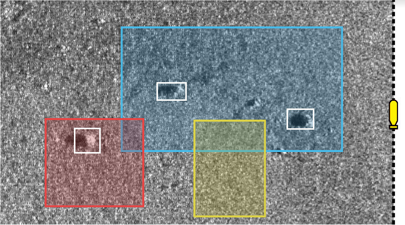
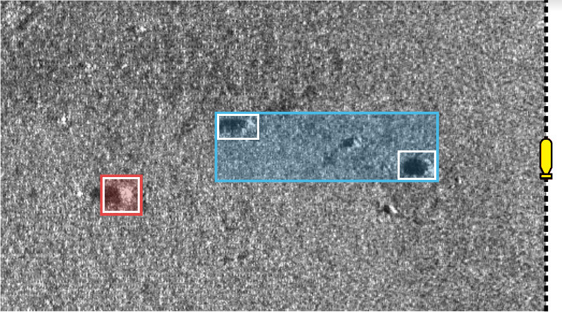
Fig. 32 Illustration of the constellation contractor, before and after the contraction step. The set \(\mathbb{M}\) of landmarks is depicted by white boxes. Colored boxes depict several cases of \([\mathbf{a}]\). In this example, the red perception leads to a reliable identification since the box contains only one item of \(\mathbb{M}\). We recall that the sonar image in background is not involved in this contraction: it is only used for understanding the application of this contractor. Here, the operator is reliable as it does not remove any significant rock.

The definition of the contractor is given by:

\[\mathcal{C}_\mathbb{M}\left(\left[\mathbf{a}\right]\right)=\bigsqcup_{j=1}^{\ell}\big(\left[\mathbf{a}\right]\cap[\mathbf{m}_{j}]\big),\]

where \(\bigsqcup\), called squared union, returns the smallest box enclosing the union of its arguments.

Exercise

D.1. We can now build our own contractor class. To do it, we have to derive the class Ctc that is common to all contractors. You can start from the following new class:

PythonC++

class MyCtc(Ctc):

  def __init__(self, M_):
    Ctc.__init__(self, 2) # the contractor acts on 2d boxes
    self.M = M_           # attribute needed later on for the contraction

  def contract(self, a):

    # Insert contraction formula here (question D.2)

    return a

(you may continue the code from the previous Lesson C)

Note that:

• M represents the set \(\mathbb{M}\), made of 2d IntervalVector objects;

• a (in .contract()) is the box \([\mathbf{a}]\) (2d IntervalVector) to be contracted.

D.2. Propose a simple implementation of the method .contract() for contracting \([\mathbf{a}]\) as:

\[\mathcal{C}_\mathbb{M}\left(\left[\mathbf{a}\right]\right)=\bigsqcup_{j=1}^{\ell}\big(\left[\mathbf{a}\right]\cap[\mathbf{m}_{j}]\big)\]

The user manual may help you to compute operations on sets such as unions or intersections, appearing in the formula. Note that you cannot change the definition of the .contract() method.

D.3. Test your contractor with:

• a set \(\mathbb{M}=\big\{(1.5,2.5)^\intercal,(3,1)^\intercal,(2,2)^\intercal,(2.5,3)^\intercal,(3.5,2)^\intercal,(4,1)^\intercal,(1.5,0.5)^\intercal\big\}\), all boxes inflated by \([-0.05,0.05]\);

• three boxes to be contracted: \([\mathbf{a}^1]=([1.25,3],[1.6,2.75])^\intercal\), \([\mathbf{a}^2]=([2,3.5],[0.6,1.2])^\intercal\), and \([\mathbf{a}^3]=([1.1,3.25],[0.2,1.4])^\intercal\).

You can try your contractor with the following code:

PythonC++

# M = [ ...
for Mi in M:
  Mi.inflate(0.05)

# a1 = IntervalVector([ ...
# a2 = IntervalVector([ ...
# a3 = IntervalVector([ ...

ctc_constell = MyCtc(M)
cn = ContractorNetwork()

cn.add(ctc_constell, [a1])
cn.add(ctc_constell, [a2])
cn.add(ctc_constell, [a3])

cn.contract()

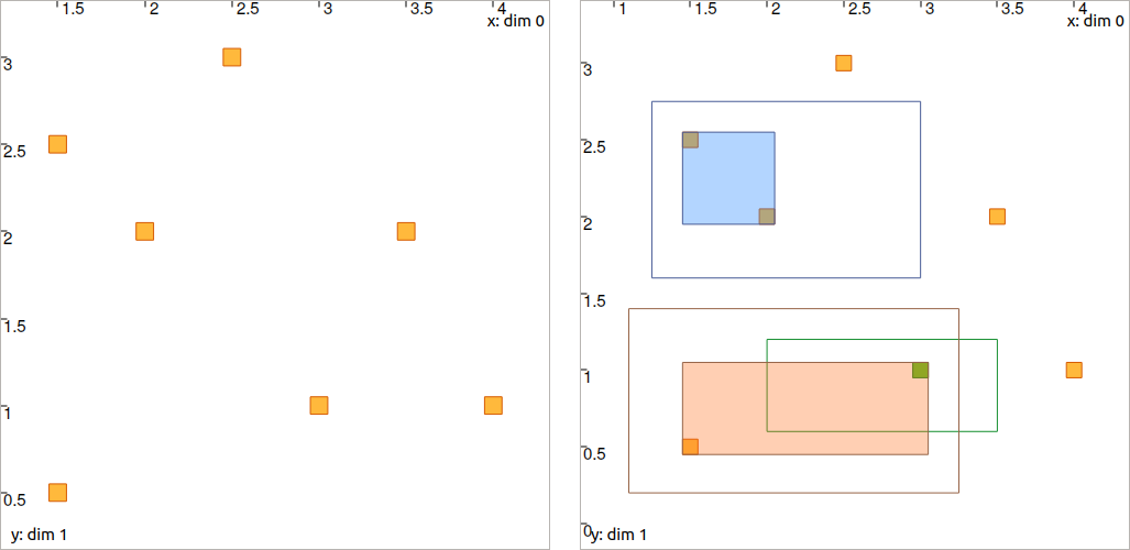
Fig. 33 Expected result for Question D.3 (you may verify your results only by printing boxes values). Non-filled boxes are initial domains before contraction. Filled boxes are contracted domains. The green one, \([\mathbf{a}^3]\), is identified since it contains only one item of the constellation \(\mathbb{M}\): there is no ambiguity about the constellation point represented by the box \([\mathbf{a}^3]\).

Numerical results are given:

[a1]: ([1.45, 2.05] ; [1.95, 2.55])    (blue box)
[a2]: ([2.95, 3.05] ; [0.95, 1.05])    (green box)
[a3]: ([1.45, 3.05] ; [0.45, 1.05])    (red box)

Application for localization

This contractor is really simple, but it will help us to solve more complex problems.

We now have all the material to solve the full problem of state estimation with data association.

We will localize the robot in the map \(\mathbb{M}\) created in Question D.3.

Exercise

D.4. In your code, define a robot with the following pose \(\mathbf{x}=\left(2,1,\pi/6\right)^\intercal\) (the same as in Lesson C).

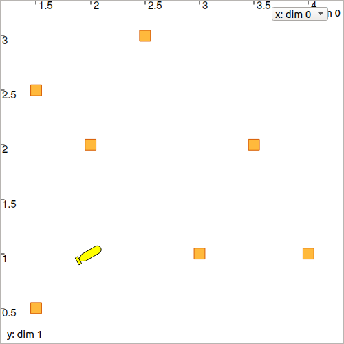
D.5. Display the robot and the landmarks in a graphical view with:

PythonC++

beginDrawing()

fig_map = VIBesFigMap("Map")
fig_map.set_properties(100,100,500,500)
fig_map.draw_vehicle(x_truth,0.5)
for Mi in M:
  fig_map.draw_box(Mi, "red[orange]")

# Draw the result of next questions here

fig_map.axis_limits(fig_map.view_box(), True, 0.1)

You should obtain this result.

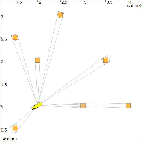
D.6. We will generate a set of range-and-bearing measurements made by the robot. For this, we will reuse a function of Lesson B:

PythonC++

v_obs = DataLoader.generate_static_observations(x_truth, M, False)

where x_truth is the actual state vector of the robot and M the set of landmarks \(\mathbb{M}\). The returned value v_obs is a vector of [range]×[bearing] interval values.

Display the measurements v_obs in the view with .draw_pie(), as we did in the previous lesson. You should obtain a figure similar to this one:

You can easily add uncertainties on these measurements, for instance with:

PythonC++

# Adding uncertainties on the measurements
for obs in v_obs:
  obs[0].inflate(0.02) # range
  obs[1].inflate(0.02) # bearing

State estimation without data association

We will go step by step and not consider the data association problem for the moment.

We will first reuse the Contractor Network developed in the previous Lesson for range-and-bearing localization, and apply it on this set of observations.

Exercise

D.7. With a Contractor Network, perform the state estimation of the robot (the contraction of \([\mathbf{x}]\)) by considering simultaneously all the observations. You can reuse the CN previously implemented in Lesson C for this purpose.

We will assume that:

• the identity (the position) of the related landmarks is known;

• the heading \(x_3\) of the robot is known.

PythonC++

# Define contractors
# ...

cn = ContractorNetwork()

for i in range(0,len(v_obs)): # for each measurement

  # Define intermediate variables
  # ...

  # Add contractors and related domains
  # ...

  # Note: v_obs[i] is a 2d vector [y^i]
  # Note: M[i] is a 2d box of M

cn.contract()

If you are using C++, please read the paragraph related to intermediate variables in C++, at the end of this page.

In the code, the identity of each landmark is known in the sense that a measurement v_obs[i] refers to a landmark M[i].

D.8. Display the resulted contracted box \([\mathbf{x}]\) with:

PythonC++

fig_map.draw_box(x.subvector(0,1)) # displays ([x_1],[x_2])

You should obtain this result in black (considering uncertainties proposed in Question D.6):

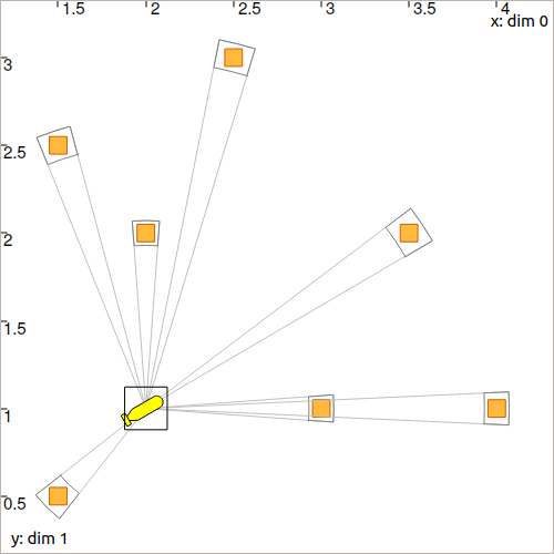
Fig. 34 Range-and-bearing static localization, with several observations of identified landmarks.

State estimation with data association

We now assume that the identities of the landmarks are not known. This means that the M[i] variables will not appear anymore in the resolution of the problem, except for creating the constellation contractor.

Exercise

D.9. Outside the resolution part, we create a list of boxes for representing possible identities of the landmarks for each measurement.

PythonC++

# Association set (possible identities)
m = [IntervalVector(2) for _ in v_obs] # unknown associations for each observation

Each m[i] object is a 2d box corresponding to the \(\mathbf{m}^i\) vector of the equations in the above Section Formalism.

D.10. Update the Contractor Network for solving the state estimation together with the data association problem. The CN should now involve the m[i] objects as well as the new contractor you developed in the Section The constellation constraint and its contractor.

PythonC++

ctc_asso = MyCtc(M)

# ...

cn.add(ctc_asso, [m[i]])

We recall that one contractor can be added to the CN several times together with different domains.

You should obtain exactly the same result as in Question D.8.

D.11. Same result means that the data association worked: each measurement has been automatically associated to the correct landmark without ambiguity.

We can now look at the set m containing the associations. If one \([\mathbf{m}^i]\) contains only one item of \(\mathbb{M}\), then it means that the landmark of the measurement \(\mathbf{y}^i\) has been identified.

We will draw a point in the middle of each \([\mathbf{m}^i]\) that contains only one item of \(\mathbb{M}\).

In Question D.3, we defined \(\mathbb{M}\) as a set of boxes with a width of \(2\times 0.05\). Then, if one box \([\mathbf{m}^i]\) has a maximal diameter that is less than \(0.1\), it means that it contains one single item of \(\mathbb{M}\).

PythonC++

for mi in m:
  if mi.max_diam() <= 0.10001: # if identified
    fig_map.draw_circle(mi[0].mid(), mi[1].mid(), 0.02, "blue[blue]")

Expected result:

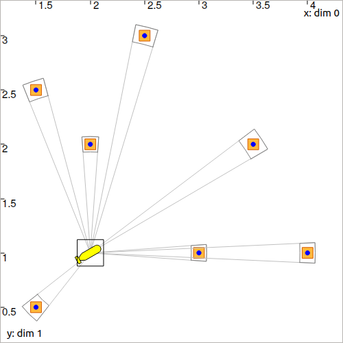
Fig. 35 All the boxes have been identified.

Conclusion

This association has been done only by merging all information together. We define contractors from the equations of the problem, and let the information propagate in the domains. This has led to a state estimation solved concurrently with a data association.

In the next lessons, we will go a step further by making the robot move. This will introduce differential constraints, and a new domain for handling uncertain trajectories: tubes.

Underwater application

We could apply this solver on actual data, such as the underwater application presented in the introduction of this lesson. The identification of the rocks on the seafloor would be done by the fusion of all data, without image processing. The same algorithm also provides a reliable way to gather different views of a same object, without using data processing.

This topic of data association with underwater robotics has been the subject of a paper proposed for this ICRA 2020 conference:

Set-membership state estimation by solving data association

Simon Rohou, Benoît Desrochers, Luc Jaulin, ICRA 2020

Download the paper

Here is a video providing an overview of the problem and how to solve it. This is mainly the object of this Lesson D and the next one, that will deal with the dynamics of the robot.

End of second step!

That’s about all for this second step.

See you next step for discovering tubes!

Appendix

Important

The case of intermediate variables in C++.

In C++, if we create intermediate variables in a different block of code than the .contract() method, then the C++ variables are destroyed at the end of their block and so the CN lose the reference to them. For instance:

ContractorNetwork cn;
CtcFunction ctc_plus(Function("a", "b", "c", "b+c-a"));
Interval x(0,1), y(-2,3);

if(/* some condition */)
{
  Interval a(1,20);
  cn.add(ctc_plus, {x, y, a}); // constraint x+y=a
} // 'a' is lost here

cn.contract(); // segmentation fault here

Instead, we must create the domains inside the CN object in order to keep it alive outside the block. This can be done with the method .create_interm_var():

ContractorNetwork cn;
CtcFunction ctc_plus(Function("a", "b", "c", "b+c-a"));
Interval x(0,1), y(-2,3);

if(/* some condition */)
{
  Interval& a = cn.create_interm_var(Interval(1,20));
  cn.add(ctc_plus, {x, y, a});
} // 'a' is not lost

cn.contract(); // the contraction works on [x], [y] and [a] that still exists

Therefore, the following function:

IntervalVector& d = cn.create_interm_var(IntervalVector(2));

creates for instance an intermediate 2d variable with a 2d box domain: \([\mathbf{d}]=[-\infty,\infty]^2\). Its argument defines the type of domain to be created (Interval, IntervalVector, etc.).

Technically, create_interm_var() returns a C++ reference (in the above example, of type IntervalVector&). The reference is an alias on the intermediate variable, that is now inside the Contractor Network. It can be used in the same way as other variables involved in the CN.