See also
This manual refers to Codac v1, but a new v2 implementation is currently in progress… an update of this manual will be available soon. See more.
CtcPolar: \(\big(x=\rho\cos\theta~;y=\rho\sin\theta\big)\)
The \(\mathcal{C}_{\textrm{polar}}\) contractor is mainly used in robotics to express a range-and-bearing constraint. It can be seen as an extension of the previously presented \(\mathcal{C}_{\textrm{dist}}\) enriched with the bearing information. However, its implementation does not stand on the \(\mathcal{C}_{\mathbf{f}}\) contractor presented in the beginning of this chapter. The implementation of \(\mathcal{C}_{\textrm{polar}}\) is minimal and originally comes from the pyIbex library.
Definition
Important
ctc.polar.contract(x, y, rho, theta)
ctc::polar.contract(x, y, rho, theta);
Optimality
This contractor is optimal.
Example
Suppose that we want to estimate the distance \(d^i\) and angle \(\theta^i\) (bearing) between a vector \(\mathbf{x}=(0,0)^\intercal\) and a vector \(\mathbf{b}^i\), \(i\in\{1,2,3\}\).
We define domains (intervals and boxes):
\([\mathbf{x}]=[0,0]^2\)
\([\mathbf{b}^1]=[1.5,2.5]\times[4,11]\), \([d^1]=[7,8]\), \([\theta^1]=[0.6,1.45]\)
\([\mathbf{b}^2]=[3,4.5]\times[8,10.5]\), \([d^2]=[9,10]\), \([\theta^2]=[1.15,1.2]\)
\([\mathbf{b}^3]=[5,6.5]\times[6.5,8]\), \([d^3]=[10,11]\), \([\theta^3]=[0.8,1]\)
x = IntervalVector(2,Interval(0))

d = [Interval(7,8), Interval(9,10), Interval(10,11)]

theta = [Interval(0.6,1.45), Interval(1.15,1.2), Interval(0.8,1)]

b = [IntervalVector([[1.5,2.5],[4,11]]), \
     IntervalVector([[3,4.5],[8,10.5]]), \
     IntervalVector([[5,6.5],[6.5,8]])]
IntervalVector x(2,0.);

Interval d1(7.,8.), theta1(0.6,1.45);
IntervalVector b1{{1.5,2.5},{4,11}};

Interval d2(9.,10.), theta2(1.15,1.2);
IntervalVector b2{{3,4.5},{8,10.5}};

Interval d3(10.,11.), theta3(0.8,1.);
IntervalVector b3{{5,6.5},{6.5,8}};
Calls to \(\mathcal{C}_{\textrm{polar}}\) will allow the contraction of the \([\mathbf{b}^i]\), \([d^i]\) and \([\theta^i]\):
ctc_polar = CtcPolar()

for i in range(0,3):
  ctc_polar.contract(b[i][0], b[i][1], d[i], theta[i])
  ctc_polar.contract(b[i][0], b[i][1], d[i], theta[i])
  ctc_polar.contract(b[i][0], b[i][1], d[i], theta[i])

# note that we could also use directly the ctc.polar object already available
CtcPolar ctc_polar;

ctc_polar.contract(b1[0], b1[1], d1, theta1);
ctc_polar.contract(b2[0], b2[1], d2, theta2);
ctc_polar.contract(b3[0], b3[1], d3, theta3);

// note that we could also use directly the ctc::polar object already available
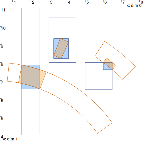
Fig. 17 Illustration of several contracted boxes and pies with the above ctc_polar contractor. The blue boxes \([\mathbf{b}^i]\) have been contracted as well as the pies \([d^i]\times[\theta^i]\).
Note
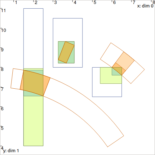
CtcFunction contractor to express the constraint, but the results would not have been optimal. This means that the resulting intervals would not perfectly size the set of feasible values. The figure on the right shows off the pessimism of such alternative.