The SepImage separator

Main author: Maël Godard

Definition

Consider a set \(\mathbb{X}\subset\mathbb{R}^n\) and a function \(\mathbf{f}:\mathbb{R}^n\to\mathbb{R}^p\). The initial set \(\mathbb{X}\) is provided through a contractor, while its boundary is described by a gnomonic atlas. The function \(\mathbf{f}\) is provided as an AnalyticFunction, allowing interval evaluations of its image.

The SepImage separator handles the image set \(\mathbf{f}(\mathbb{X})\) by separating boxes \([\mathbf{y}]\in\mathbb{IR}^p\) with respect to the constraint \(\mathbf{y}\in\mathbf{f}(\mathbb{X})\).

Construction and basic usage

The SepImage relies on a boundary approach to compute the image set. The boundary of the initial set needs to be covered by a gnomonic atlas. To compute the image of the boundary, the parameter box \(\left[-1,1\right]^m\) can be subdivided up to a size \(\epsilon\) and the image of each resulting box is computed. Note that if one chooses to take \(\epsilon=2\), only one computation will be done per chart of the atlas.

Once this image of the boundary has been computed, the SepImage needs a way to characterize if a point is inside or outside of the image set. To do so, it looks for an antecedent of the point in the initial set. An additional contractor on the initial set is then required.

The typical workflow is:

1. Define analytic variables (scalar, vector, matrix) associated with the domain of the function.

2. Build an AnalyticFunction.

3. Define a gnomonic atlas on the boundary of the initial set.

4. Define a contractor for this same initial set.

5. Instantiate SepImage with the atlas, the function, the resolution \(\epsilon\) and the contractor.

6. Contract an input box \([\mathbf{y}]\) or pave the separator in the image space.

Example

Consider that we want to construct a separator on the image of the unit disk by the function

\[\begin{split}\mathbf{f}(\mathbf{x})= \left( \begin{array}{c} 3(x_{1}+1)\\ x_{2}+ 0.5\sin (3 x_{1}) \end{array} \right)\end{split}\]

This function can be constructed in codac as follows

PythonC++

y = VectorVar(2)
f = AnalyticFunction([y], [3.*(y[0]+1),y[1]+0.5*sin(3.*y[0])])

We then need a contractor for the unit disk, and a gnomonic atlas for its boundary (the unit circle). For the atlas, the image of \(\left[-1,1\right]\) by the function

\[\begin{split}\psi_{0} = \left( \begin{array}{c} \cos\left(x\cdot\frac{\pi}{2}\right)\\ \sin\left(x\cdot\frac{\pi}{2}\right) \end{array} \right)\end{split}\]

is half of the unit circle. The other half can be obtained with a rotation of \(\pi\) rad. Such atlas is constructed in Codac as follows:

PythonC++

# {psi0,Sigma} is a gnomonic atlas of the box [-1,1]^2
X = VectorVar(1)
psi0 = AnalyticFunction([X],[cos(X[0]*PI/2.),sin(X[0]*PI/2.)])

id = OctaSym([1,2])
s = OctaSym([-1,-2])

Sigma = [id,s]

In this example, the constraint on the initial set can be seen as a distance constraint. It can be treated as an inversion as follows :

PythonC++

h = AnalyticFunction([y],sqrt(sqr(y[0])+sqr(y[1])))
ctc_in = CtcInverse(h,Interval(0,1))

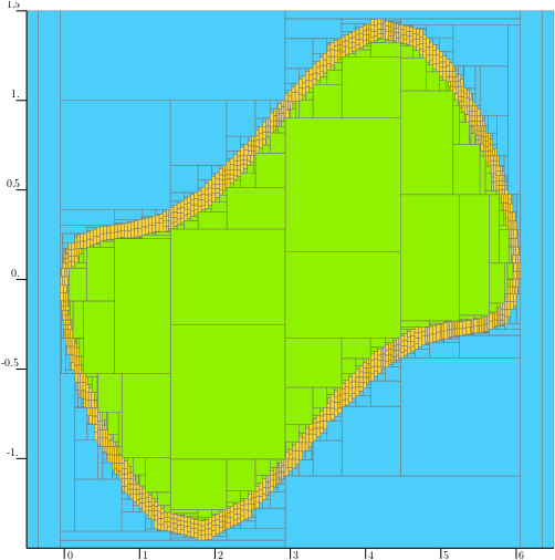
The separator can then be constructed and used, for example with a paver to get both an inner and an outer approximation of the image set. The resulting paving is shown in the next figure.

PythonC++

sep = SepImage(f,psi0,Sigma,0.125,ctc_in)
DefaultFigure.pave([[-0.5,6.5],[-1.5,1.5]],sep,0.05)

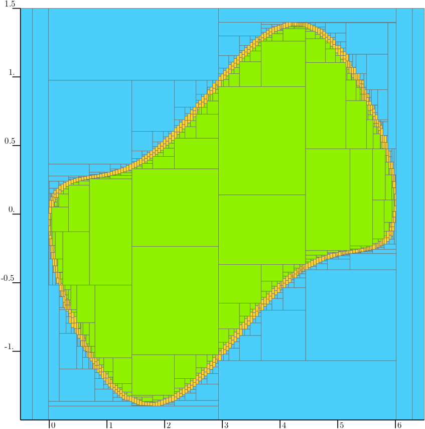
With a finer resolution (i.e., a smaller \(\epsilon\)), the approximation provided by the separator improves, as shown in the following figure.

PythonC++

sep = SepImage(f,psi0,Sigma,0.0625,ctc_in)
DefaultFigure.pave([[-0.5,6.5],[-1.5,1.5]],sep,0.05)

A more complex example is available on the public GitHub repository. It treats the topic of the explored area, which is a classical problem in robotics.

• Python version

• C++ version