The SlicedTube class

Main author: Simon Rohou

A SlicedTube is a tube defined over a shared TDomain. For each temporal slice stored in the temporal partition, the tube owns one Slice object storing its codomain over that temporal support. The codomain type is typically Interval or IntervalVector, or any domain type defined by the user. The same temporal domain can be shared by many tubes.

Creating sliced tubes

In Codac C++, SlicedTube is a generic class template SlicedTube<T>. The codomain type T is not restricted to intervals or boxes: in principle, any domain type compatible with the sliced-tube API can be used.

In practice, the most common sliced-tube types are:

• SlicedTube<Interval>,

• SlicedTube<IntervalVector>,

• SlicedTube<IntervalMatrix>.

These standard tube types are also the ones exposed in the Python and Matlab bindings.

In C++, template argument deduction is available for the constructors based on the arguments. In the examples below, comments make the deduced type explicit when useful.

A sliced tube can be created from:

• a constant codomain,

• an analytic function of one scalar variable,

• a sampled or an analytic trajectory,

• or another sliced tube (copy constructor).

PythonC++

td = create_tdomain([0,10], 0.1, True)

# Sliced tube from interval-type codomains
x = SlicedTube(td, Interval(-1,1))
y = SlicedTube(td, IntervalVector(2))
z = SlicedTube(td, IntervalMatrix(2,2))

# From an analytic function
t = ScalarVar()
f = AnalyticFunction([t], sin(t))
xf = SlicedTube(td, f)

# From an analytic trajectory or sampled trajectory
at = AnalyticTraj([0,10], AnalyticFunction([t],cos(t)))
st = AnalyticTraj([0,10], AnalyticFunction([t],cos(t)+t/10)).sampled(1e-2)
xu = SlicedTube(td,at) | SlicedTube(td,st) # union (hull) of tubes

fig.plot_tube(xf, [Color.dark_blue(),Color.light_gray()])
fig.plot_tube(xu, [Color.dark_blue(),Color.light_gray()])

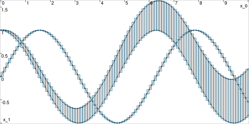
Created tubes \([x_f](\cdot)=[\sin(\cdot),\sin(\cdot)]\) and \([x_u](\cdot)=[\cos(\cdot),\cos(\cdot)+\frac{\cdot}{10}]\), made of 100 slices.

Basic properties

A sliced tube exposes:

• size() for the codomain dimension,

• shape() for matrix-like codomain shapes,

• tdomain() and t0_tf() from the base classes,

• nb_slices() for the number of temporal elements,

• codomain() for the global codomain hull,

• volume() for the sum of non-gate slice volumes,

• is_empty() and is_unbounded().

Accessing slices and iterating

You can access the first and last slices directly:

• first_slice()

• last_slice()

and you can retrieve a slice from a temporal-domain iterator or from a TSlice pointer. The class also defines custom iterators so that iterating on a SlicedTube yields application-level Slice objects rather than raw TSlice objects.

PythonC++

td = create_tdomain([0,3])
x = SlicedTube(td, IntervalVector(2))
x.set([[1,5],[-oo,2]], [0,1])
x.set([[2,8],[-oo,3]], [1,2])
x.set([[6,9],[-oo,4]], [2,3])

s0 = x.first_slice()
s1 = s0.next_slice()

for s in x:
  print(s.t0_tf(), s.codomain())

Setting values and refining the partition

A sliced tube can be updated globally or locally:

• set(codomain) sets all slices to the same codomain,

• set(codomain, t) sets the value at one time instant,

• set(codomain, [ta,tb]) sets all temporal elements intersecting an interval,

• set_ith_slice(codomain, i) sets one stored slice by index.

The key point is that local assignments may refine the underlying TDomain. For example, setting a value at one scalar time creates an explicit gate if necessary. Similarly, setting a value over an interval may create new temporal boundaries at the interval endpoints.

Note

Because the temporal domain is shared, such refinements are structural operations. If several tubes share the same TDomain, all of them will observe the new partition.

PythonC++

td = create_tdomain([0,2], 1.0, False) # False: without gates

x = SlicedTube(td, Interval(0,1))
v = SlicedTube(td, Interval(-1,1))

print(x)            # outputs [0,2]->[0,1], 2 slices
print(v)            # outputs [0,2]->[0,1], 2 slices

n = td.nb_tslices() # 2: [0,1],[1,2]
x.set([0.5,1], 1.3) # local update, will refine the partition at t=1.3
m = td.nb_tslices() # now 4: [0,1],[1,1.3],[1.3],[1.3,2]

print(x)            # outputs [0,2]->[-1,1], 4 slices
print(v)            # outputs [0,2]->[-1,1], 4 slices (v is also impacted by x.set(..))

Evaluation

A sliced tube \([x](\cdot)\) can be evaluated over a temporal interval \([t]\) with x(t). The implementation walks through all relevant temporal slices, evaluates each local slice, and unions the results. If the query interval is not included in the temporal domain, the result is the unbounded value of the codomain type (for interval tubes: \([-\infty,\infty]\)).

When a derivative tube v is available, the overload x(t,v) uses per-slice derivative-aware evaluation and unions the resulting enclosures. This is available for Interval and IntervalVector codomain types.

PythonC++

td = create_tdomain([0,3], 1.0, False)
x = SlicedTube(td, Interval())

x.set([1,5], [0,1])
x.set([2,8], [1,2])
x.set([6,9], [2,3])

x(0.5)      # [1,5]
x(1.5)      # [2,8]
x([0,3])    # [1,9]
x(-1.0)     # [-oo,oo]

# No explicit gates: boundary values come from adjacent-slice intersections
x(1.0)      # [2,5]
x(2.0)      # [6,8]
x(3.0)      # [6,9]

Inversion

The inversion of a sliced tube \([x](\cdot)\), denoted \([x]^{-1}([y])\), is defined by

\[[x]^{-1}([y]) = \left\{\, t \mid [x](t)\cap [y]\neq\varnothing \,\right\} = \bigcup_{y\in [y]} \left\{\, t \mid y\in [x](t) \,\right\}.\]

It is illustrated by the figure below. Intuitively, the inversion returns the set of time values whose image under \([x](\cdot)\) intersects the target set \([y]\).

Depending on the overload, the invert() methods

• invert(y, t=[...])

• invert(y, v_t, t=[...])

• invert(y, v, t=[...])

• invert(y, v_t, v, t=[...])

return either:

• one interval enclosing the union of all preimages,

• or the different connected components of the inversion in a vector of Interval objects.

When a derivative tube v is provided, Codac uses derivative information slice by slice in order to compute sharper inverse images.

The following example computes the different connected components of the inversion \([x]^{-1}([0,0.2])\) over a temporal subdomain, and then draws their projections in red.

PythonC++

v_t = []
y = Interval(0,0.2)
x.invert(y,v_t)

for t in v_t:
  z = cart_prod(t,y)
  DefaultFigure.draw_box(z, Color.red())

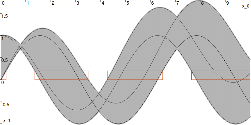
Example of tube inversion for a given tube \([x](\cdot)\). The red boxes correspond to the connected components of \([x]^{-1}([0,0.2])\).

group Inversion of sliced tubes

Functions

inline Interval invert(const T &y, const Interval &t) const

Returns the interval inversion \(\left[[x]^{-1}([y])\right]\).

If the inversion results in several pre-images, their union is returned.

Parameters:

• y – interval codomain

• t – (optional) temporal domain on which the inversion will be performed

Returns:

the hull of \([x]^{-1}([y])\)

inline void invert(const T &y, std::vector<Interval> &v_t, const Interval &t) const

Computes the set of continuous values of the inversion \([x]^{-1}([y])\).

Parameters:

• y – interval codomain

• v_t – vector of the sub-tdomains \([t_k]\) for which \(\forall t\in[t_k] \mid x(t)\in[y], x(\cdot)\in[x](\cdot)\)

• t – (optional) temporal domain on which the inversion will be performed

inline Interval invert(const T &y, const SlicedTube<T> &v, const Interval &t) const

Returns the optimal interval inversion \(\left[[x]^{-1}([y])\right]\).

The knowledge of the derivative tube \([v](\cdot)\) allows a finer inversion. If the inversion results in several pre-images, their union is returned.

Parameters:

• y – interval codomain

• v – derivative tube such that \(\dot{x}(\cdot)\in[v](\cdot)\)

• t – (optional) temporal domain on which the inversion will be performed

Returns:

hull of \([x]^{-1}([y])\)

inline void invert(const T &y, std::vector<Interval> &v_t, const SlicedTube<T> &v, const Interval &t) const

Computes the set of continuous values of the optimal inversion \([x]^{-1}([y])\).

The knowledge of the derivative tube \([v](\cdot)\) allows finer inversions.

Parameters:

• y – interval codomain

• v_t – vector of the sub-tdomains \([t_k]\) for which \(\forall t\in[t_k] \mid x(t)\in[y], x(\cdot)\in[x](\cdot), \dot{x}(\cdot)\in[v](\cdot)\)

• v – derivative tube such that \(\dot{x}(\cdot)\in[v](\cdot)\)

• t – (optional) temporal domain on which the inversion will be performed

Tube operations

Standard pointwise operations are available on sliced tubes and are applied slice by slice.

For two tubes, binary operators require both operands to share the same TDomain. This makes tube expressions easy to combine once the tubes have been built on a common temporal support.

The following operators are available:

• union and intersection: | and &,

• arithmetic operations: +, -, *, /,

• in-place variants: |=, &=, +=, -=, *=, /=.

For scalar interval tubes, several usual nonlinear functions are also provided, including sqr, sqrt, pow, exp, log, sin, cos, tan, atan2, abs, min, max, sign, floor and ceil.

PythonC++

td = create_tdomain([0,2], 1.0, False)

x = SlicedTube(td, Interval(1,2))
y = SlicedTube(td, Interval(-1,3))

z_add = x + y  # addition of two tubes
z_mul = 2 * x  # multiplication by a scalar/interval
z_hul = x | y  # hull (union) of two tubes
z_int = x & y  # intersection of two tubes

u = sin(x) + exp(y)

For vector-valued codomains, pointwise arithmetic is also available. In particular, the product of a matrix tube and a vector tube returns a vector tube.

PythonC++

A = SlicedTube(td, IntervalMatrix(2,2))
b = SlicedTube(td, IntervalVector(2))

y = A * b

Integration and primitives

Reliable integral computations are available on tubes.

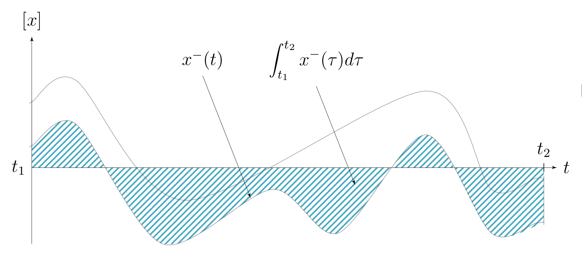
Hatched part depicts \(\int_{a}^{b}x^-(\tau)d\tau\), the lower bound of \(\int_{a}^{b}[x](\tau)d\tau\).

The computation is reliable even for tubes defined from analytic functions, because it stands on the tube’s slices that are reliable enclosures. The result is an outer approximation of the integral of the tube represented by these slices:

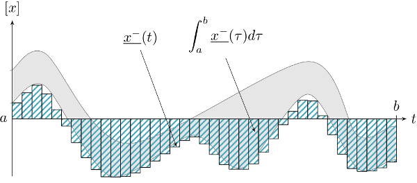
Outer approximation of the lower bound of \(\int_{a}^{b}[x](\tau)d\tau\).

group Integration and primitive operations on sliced tubes

The following methods are valid for tubes defined for Interval or IntervalVector codomains. The returned values are integral enclosures of same type (respectively, Interval or IntervalVector).

Functions

T integral(const Interval &t) const

Returns an enclosure of the integrals of this tube from \(t_0\) to \([t]\).

This method computes an enclosure of

\[ \left\{ \int_{t_0}^{\tau} [x](s)\,ds \;\middle|\; \tau\in[t] \right\}. \]

It is obtained from partial_integral(t) by taking the hull between the lower bound of the lower enclosure and the upper bound of the upper enclosure.

Parameters:

t – temporal interval \([t]\)

Returns:

enclosure of the integrals of this tube over t

T integral(const Interval &t1, const Interval &t2) const

Returns an enclosure of the integrals of this tube between the time intervals \([t_1]\) and \([t_2]\).

This method computes an enclosure of

\[ \left\{ \int_{\tau_1}^{\tau_2} [x](s)\,ds \;\middle|\; \tau_1\in[t_1],\ \tau_2\in[t_2] \right\}. \]

The result is obtained by subtracting the partial integral enclosures at t1 and t2.

Parameters:

• t1 – first temporal interval \([t_1]\)

• t2 – second temporal interval \([t_2]\)

Returns:

enclosure of the integrals of this tube between t1 and t2

std::pair<T, T> partial_integral(const Interval &t) const

Returns lower and upper enclosures of the integrals of this tube \([x](\cdot)=[x^-(\cdot),x^+(\cdot)]\) from \(t_0\) to \([t]\).

This method returns a pair \(([p^-],[p^+])\) such that:

\[ [p^-]\supset \left\{ \int_{t_0}^{\tau} x^-(s)\,ds \;\middle|\; \tau\in[t] \right\} \mathrm{~~and~~} [p^+]\supset \left\{\int_{t_0}^{\tau} x^+(s)\,ds \;\middle|\; \tau\in[t] \right\}. \]

This representation preserves more information than integral(t), which only returns the hull of these partial integral bounds.

Parameters:

t – temporal interval \([t]\)

Returns:

pair of lower and upper partial integral enclosures over t

std::pair<T, T> partial_integral(const Interval &t1, const Interval &t2) const

Returns lower and upper enclosures of the integrals of this tube \([x](\cdot)=[x^-(\cdot),x^+(\cdot)]\) between \([t_1]\) and \([t_2]\).

This method returns a pair obtained by subtracting the partial integral enclosures at t1 from those at t2. The returned pair \(([p^-],[p^+])\) is such that:

\[ [p^-]\supset \left\{ \int_{\tau_1}^{\tau_2} x^-(s)\,ds \;\middle|\; \tau_1\in[t_1],\ \tau_2\in[t_2] \right\}, \]

and

\[ [p^+]\supset \left\{\int_{\tau_1}^{\tau_2} x^+(s)\,ds \;\middle|\; \tau_1\in[t_1],\ \tau_2\in[t_2] \right\}. \]

Parameters:

• t1 – first temporal interval \([t_1]\)

• t2 – second temporal interval \([t_2]\)

Returns:

pair of lower and upper enclosures of the integrals

inline SlicedTube<T> primitive() const

Returns a primitive of this tube with zero initial condition.

This is a shorthand for primitive(x0) with \(x_0 = 0\).

In other words, the returned tube encloses solutions of

\[ \dot{p}(\cdot) \in [x](\cdot), \qquad p(t_0)=0. \]

Returns:

primitive tube with zero initial condition

inline SlicedTube<T> primitive(const T &x0) const

Returns a primitive of this tube with prescribed initial condition.

This method constructs a tube p on the same temporal domain as this tube, imposes the initial condition \(p(t_0)=x_0\), and contracts p with this tube through the derivative relation using CtcDeriv.

In other words, the returned tube encloses solutions of

\[ \dot{p}(\cdot) \in [x](\cdot), \qquad p(t_0)=x_0. \]

Note

The current implementation may create an explicit gate at the initial time \(t_0\) if it is not already present in the temporal partition.

Parameters:

x0 – initial condition at \(t_0\)

Returns:

primitive tube satisfying the prescribed initial condition

Inflation, extraction, and algebraic helpers

A sliced tube can be inflated either by a constant radius or by a time-varying sampled radius. Inflation is performed in place.

PythonC++

x.inflate(0.2) # constant inflation

rad = SampledTraj({0.0:0.1, 1.0:0.3, 2.0:0.2})
x.inflate(rad) # time-varying inflation radius

For vector-valued tubes, the API also provides convenient extraction operators:

• x[i] returns the \(i\)-th scalar component as a SlicedTube,

• x.subvector(i,j) returns a subvector tube.

The extracted tubes keep the same temporal partition as the original one.

PythonC++

# Component and subvector extraction
x0 = x[0]
x12 = x.subvector(1,2)

Involving a tube in an analytic expression

The method .as_function() wraps a sliced tube as an analytic operator so that it can be embedded inside analytic expressions. This is a convenient bridge between the tube API and the analytic-expression API, see the section on temporal operators for its use.